MacKenzie, I. S. (2018). Fitts' law. In K. L. Norman & J. Kirakowski (Eds.), Handbook of human-computer interaction, pp. 349-370. Hoboken, NJ: Wiley. doi:10.1002/9781118976005 [PDF] [software]
Fitts' Law
I. Scott MacKenzie
York UniversityDept of Electrical Engineering and Computer Science
Toronto, Canada
mack@cse.yorku.ca
Introduction
Human movement is ubiquitous in computing. Our arms, wrists, and fingers busy themselves on keyboards, desktops, and contact-sensitive displays. And so, matching the movement limits and capabilities of humans with interaction techniques on computing systems is an important area of research in human-computer interaction (HCI). Considerable HCI research is directed at modeling, predicting, and measuring human performance. In the realm of human movement, Fitts' law is the pre-eminent model for this research.
The full spectrum of human movement applicable to Fitts' law is broader than the three examples – arms, wrists, and fingers – given in the preceding paragraph. In contexts such as gaming, virtual reality, or accessible computing, movements may also involve the torso, legs, feet, eyes, face, tongue, lip, skin, head, and so on. Notably, for each of these input modalities, there are examples where Fitts' law was used to explore the design space or to quantify human performance.
This chapter provides an overview of Fitts' law. As we shall see, Fitts' law is a model both for predicting and measuring. For predicting, Fitts' law is an equation giving the time to acquire and select a target based on the distance moved and the size of the target. For measuring, Fitts' law provides a method to quantify human performance in a single measure, "throughput". Throughput, when calculated as described later in this chapter, combines speed and accuracy in performing a target acquisition task.
We begin with background details and a brief tour of Fitts' law, and follow by describing refinements to correct flaws or to improve the model's prediction power or theoretical basis. Fitts' law evaluations of computer input techniques are more consistent in recent years due to the emergence of ISO 9241-9, an ISO standard for evaluating input devices. The Fitts' law methods used in the standard are summarized and software tools are presented that implement the methods. Since Fitts' throughput is the main performance measure for such evaluations, we also detail the calculation of throughput according to best-practice methods. We then present an example of the use of Fitts' law and ISO 9241-9 for measuring human performance. The example involves touch-based target selection on a mobile phone with a contact-sensitive display.
Background
Like many psychologists in the 1950s, Fitts was motivated to investigate whether human performance could be quantified using a metaphor from the new and exciting field of information theory. This field emerged from the work of Shannon, Wiener, and other mathematicians in the 1940s. The terms probability, redundancy, bits, noise, and channels entered the vocabulary of experimental psychologists as they explored the latest technique of measuring and modeling human behavior. Two well-known models in this vein are the Hick-Hyman law for choice reaction time (Hick, 1952; Hyman, 1953) and Fitts' law for the information capacity of the human motor system (Fitts, 1954).
Fitts' particular interest was rapid-aimed movements, where a human operator acquires or selects targets of a certain size over a certain distance. Fitts proposed a model – now "law" – that is widely used in fields such as ergonomics, engineering, psychology, and human-computer interaction. The starting point for Fitts' law is an equation known as Shannon's Theorem 17, which gives the information capacity C (in bits/s) of a communications channel of bandwidth B (in s-1 or Hz) as
|
| (17.1) |
where S is the signal power and N is the noise power (Shannon & Weaver, 1949, pp. 100-103). Fitts reasoned that a human operator that performs a movement over a certain amplitude to acquire a target of a certain width is demonstrating a "rate of information transfer" (Fitts, 1954, p. 381). In Fitts' analogy, movement amplitudes are like signals and target tolerances or widths are like noise.
Fitts proposed an index of difficulty (ID) for a target acquisition task using a log-term slightly rearranged from Eq. 17.1. Signal power (S) and noise power (N) are replaced by movement amplitude (A) and target width (W), respectively:
|
| (17.2) |
Fitts referred to the target width as the "permissible variability" or the "movement tolerance" (Fitts, 1954, p. 382). This is the region within which a movement is terminated. As with the log-term in Eq. 17.1, the units for ID are bits because the ratio within the parentheses is unitless and the log is taken to base 2.
Fitts' idea was novel for two reasons: First, it suggested that the difficulty of a target selection task could be quantified using the information metric bits. Second, it introduced the idea that the act of performing a target selection task is akin to transmitting information through a channel – a human channel. Fitts called the rate of transmission the index of performance, although today the term throughput (TP) is more common. (For consistency, the term throughput is used throughout this chapter.)
Throughput is calculated over a sequence of trials as a simple quotient. The index of difficulty (ID) of the task is the numerator and the mean movement time (MT) is the denominator:
|
| (17.3) |
With ID in bits and MT in seconds, TP has units bits per second or bits/s. A central thesis in Fitts' work is that throughput is independent of movement amplitude and target width, as embedded in ID. In other words, as ID changes (due to changes in A or W), MT changes in an opposing manner and TP remains more or less constant.
Of course, throughput is expected to be influenced by other factors, such as device, interaction property, or environment. Two devices were compared in Fitts' original experiment (see next section). In HCI, a myriad of factors, or independent variables, can be explored using Fitts' throughput as a dependent variable. Examples include "device" (mouse vs. stylus vs. trackball – see MacKenzie, Sellen, & Buxton, 1991), "dwell interval" with an eye tracker (700 ms vs. 500 ms – see Zhang & MacKenzie, 2007), or "device position" (supported vs. mobile – see MacKenzie, 2015). Throughput is particularly appealing as a dependent variable because it combines speed and accuracy in a single measure (using a technique described shortly).
Of the two uses of Fitts' law noted above – predicting and measuring – throughput exemplifies the use of Fitts' law for measuring.
Fitts' Experiments
The original investigation (Fitts, 1954) involved four experiment conditions: two reciprocal or serial tapping tasks (1-oz stylus and 1-lb stylus), a disc transfer task, and a pin transfer task. For the tapping condition, a participant moved a stylus back and forth between two plates as quickly as possible and tapped the plates at their centers (see Figure 17.1a). Fitts later devised a discrete variation of the task (Fitts & Peterson, 1964). For the discrete task, the participant selected one of two targets in response to a stimulus light (see Figure 17.1b). The tasks in Figure 17.1 are commonly called the "Fitts' paradigm". It is easy to image how to update Fitts' apparatus using contemporary computing technology.
(a)(b)
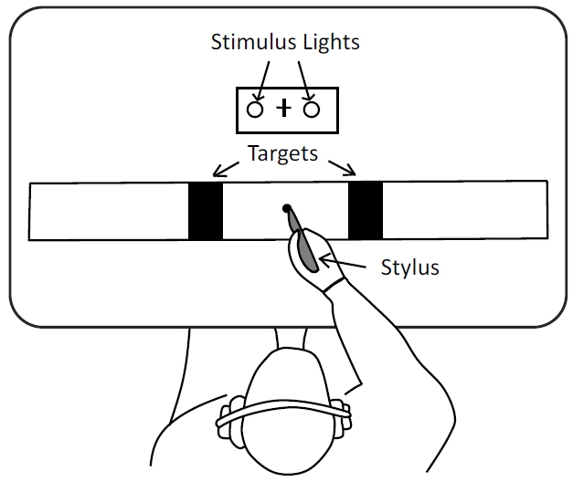
Figure 17.1. The Fitts paradigm. (a) serial tapping task (after Fitts, 1954) (b) discrete task (after Fitts & Peterson, 1964).
Fitts published summary data for his 1954 experiments, so a re-examination of his results is possible. For the stylus tapping conditions, four target amplitudes (A) were crossed with four target widths (W). For each A-W condition, participants performed two sequences of trials lasting 15 s each. (In current practice, a "sequence" is usually a specified number of trials, for instance 25, rather than a specified time interval.) The summary data for the 1-oz stylus condition are given in Table 17.1. As well as A and W, the table includes the error rate (ER), index of difficulty (ID), movement time (MT), and throughput (TP). The effective target width (We) column was added, as discussed shortly.
Table 17.1
Data from Fitts' (1954) serial tapping task experiment with a 1-oz stylus. An extra column shows the effective target width (We) after adjusting W for the percentage errors (see text).
A
(in)W
(in)We
(in)ER
(%)ID
(bits)MT
(ms)TP
(bits/s)2 0.25 0.243 3.35 4 392 10.20 2 0.50 0.444 1.99 3 281 10.68 2 1.00 0.725 0.44 2 212 9.43 2 2.00 1.020 0.00 1 180 5.56 4 0.25 0.244 3.41 5 484 10.33 4 0.50 0.468 2.72 4 372 10.75 4 1.00 0.812 1.09 3 260 11.54 4 2.00 1.233 0.08 2 203 9.85 8 0.25 0.235 2.78 6 580 10.34 8 0.50 0.446 2.05 5 469 10.66 8 1.00 0.914 2.38 4 357 11.20 8 2.00 1.576 0.87 3 279 10.75 16 0.25 0.247 3.65 7 731 9.58 16 0.50 0.468 2.73 6 595 10.08 16 1.00 0.832 1.30 5 481 10.40 16 2.00 1.519 0.65 4 388 10.31 Mean 391.5 10.10 SD 157.3 1.33
The combination of conditions in Table 17.1 yields task difficulties ranging from 1 bit to 7 bits. The mean MTs observed ranged from 180 ms (ID = 1 bit) to 731 ms (ID = 7 bits), with each mean derived from more than 600 observations over 16 participants. The standard deviation in the MT values was 157.3 ms, which is 40.2% of the mean. This is fully expected since "hard tasks" (e.g., ID = 7 bits) will obviously take longer than "easy tasks" (e.g., ID = 1 bit).
Fitts calculated throughput by dividing ID by MT (Eq. 17.3) for each task condition. The mean throughput was 10.10 bits/s. A quick glance at the TP column in Table 17.1 shows strong evidence for the thesis that the rate of information processing is relatively independent of task difficulty. Despite the wide range of task difficulties, the standard deviation of the TP values was 1.33 bits/s, which is just 13.2% of the mean.
One way to visualize the data in Table 17.1 and the independence of ID on TP is through a scatter plot showing the MT-ID point for each task condition. Figure 17.2 shows such a plot for the data in Table 17.1. The figure also includes the best-fitting line (via least-squares regression), the linear equation, and the squared correlation. The independence of ID on TP is reflected in the closeness of the points to the regression line (indicating a constant ID / MT ratio). Indeed, the fit is very good with 96.6% of the variance explained by the model.
Figure 17.2. Scatter plot and least-squares regression analysis for the data in Table 17.1.
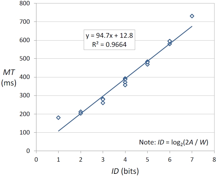
The linear equation in Figure 17.2 takes the following general form:
| MT = a + b ID | (17.4) |
The regression coefficients include an intercept a with units seconds and a slope b with units seconds per bit. (Several interesting yet difficult issues arise in interpreting the slope and intercept coefficients in Eq. 17.4. Due to space limitations, these are not elaborated here. The interested reader is directed to sections 3.4 and 3.5 in Soukoreff and MacKenzie, 2004.) Eq. 17.4 exemplifies the use of Fitts' law for predicting. This is in contrast with Eq. 17.3 which is the use of Fitts' law for measuring.
Refinements to Fitts' Law
In the years since the first publication in 1954, many changes or refinements to Fitts' law have been proposed. While there are considerations in both theory and practice, a prevailing rationale is the need for precise mathematical formulations in HCI and other fields for the purpose of measurement. One can imagine (and hope!) that different researchers using Fitts' law to examine similar phenomena should obtain similar results. This is only possible if there is general agreement on the methods for gathering and applying data.
An early motivation for altering or improving Fitts' law stemmed from the observation that the MT-ID data points curved away from the regression line, with the most deviate point at ID = 1 bit. This is clearly seen in the left-most point in Figure 17.2. In an effort to improve the data-to-model fit, Welford (1960, 1968, p. 147) introduced the following formulation:
|
| (17.5) |
This version of ID has been used frequently over the years, and in particular by Card et al. (1978) in their comparative evaluation of the computer mouse. (A re-analysis of the results reported by Card et al., 1978, are given by MacKenzie and Soukoreff, 2003, in view of a contemporary understanding of Fitts' law.) Fitts also used the Welford formulation in a 1968 paper and reported an improvement in the regression-line fit compared to the Fitts formulation (Fitts & Peterson, 1964, p. 110).
In 1989, it was shown that Fitts deduced his relationship citing an approximation of Shannon's theorem that only applies if the signal-to-noise ratio is large (Fitts, 1954, p. 388; Goldman, 1953, p. 157; MacKenzie, 1989, 1992). The signal-to-noise ratio in Shannon's theorem appears as the A-to-W ratio in Fitts' analogy. As seen in Table 17.1, the A-to-W ratio in Fitts' stylus-tapping experiment extended as low as 1:1! The variation of Fitts' index of difficulty suggested by direct analogy with Shannon's information theorem is
|
| (17.6) |
Besides the improved link with information theory, Eq. 17.6, known as the Shannon formulation, provides better correlations compared to the Fitts or Welford formulation (MacKenzie, 1989, Table 1 and Table 2; 1991, Table 4; 2013, Table 3).
An additional feature of the Shannon formulation is that ID cannot be negative. Obviously, a negative rating for task difficulty presents a serious theoretical problem. Although the prospect of a negative ID may seem unlikely, such conditions have actually been reported in the Fitts' law literature (Card et al., 1978; Crossman & Goodeve, 1983; Gillan, Holden, Adam, Rudisill, & Magee, 1990; Ware & Mikaelian, 1987). With the Shannon formulation, a negative ID is simply not possible. This is illustrated in Figure 17.3, which shows ID smoothly approaching 0 bits as A approaches 0. With the Fitts and Welford formulations, ID dips negative for small A.
Figure 17.3. With the Shannon formulation, ID approaches 0 bits as A approaches 0.

Adjustment for Accuracy
Of greater practical importance is a technique to improve the information-theoretic analogy in Fitts' law by adjusting the specified or set target width (akin to noise) according to the spatial variability in the human operator's output responses over a sequence of trials. The idea was first proposed by Crossman in 1957 in an unpublished report (cited in Welford, 1968, p. 147). Use of the adjustment was later examined and endorsed by Fitts (Fitts & Peterson, 1964, p. 110).
The output or effective target width (We) is derived from the distribution of "hits" (see MacKenzie, 1992, section 3.4; Welford, 1968, pp. 147-148). This adjustment lies at the very heart of the information-theoretic metaphor – that movement amplitudes are analogous to "signals" and that endpoint variability (viz., target width) is analogous to "noise." In fact, the information theorem underlying Fitts' law assumes that the signal is "perturbed by white thermal noise" (Shannon & Weaver, 1949, p. 100). The analogous requirement in motor tasks is a Gaussian or normal distribution of hits – a property observed by numerous researchers (e.g., Fitts & Radford, 1966; MacKenzie, 1991, p. 84; 2015; Welford, 1968, p. 154).
The experimental implication of normalizing output measures is illustrated as follows. The entropy, or information, in a normal distribution is log2((2πe)1/2σ) = log2(4.133 σ), where σ is the standard deviation in the unit of measurement. Splitting the constant 4.133 into a pair of z-scores for the unit-normal curve (i.e., σ = 1), one finds that 96% of the total area is bounded by −2.066 < z < +2.066. In other words, a condition that target width is analogous to noise is that the distribution is normal with 96% of the hits falling within the target and 4% of the hits missing the target. See Figure 17.4a. When an error rate other than 4% is observed, target width is adjusted to form the effective target width in keeping with the underlying theory.
(a)(b)
Figure 17.4. Method of adjusting target width based on the distribution of selections. (a) When 4% errors occur, the effective target width, We = W. (b) When less than 4% errors occurs, We < W.

There are two methods for determining the effective target width, the standard-deviation method and the discrete-error method. If the standard deviation of the endpoint coordinates is known, just multiply SD by 4.133 to get We. If only the percentage of errors is known, the method uses a table of z-scores for areas under the unit-normal curve. (Such a table is found in the appendix of most statistics textbooks. z-scores are also available using the NORM.S.INV function in Microsoft Excel.) Here is the method: If n percent errors are observed over a sequence of trials for a particular A-W condition, determine z such that ±z contains 100 - n percent of the area under the unit-normal curve. Multiply W by 2.066 / z to get We. As an example, if 2% errors occur on a sequence of trials when selecting a 5-cm wide target, then We = 2.066 / z × W = 2.066 / 2.326 × 5 = 4.45 cm. See Figure 17.4b. Broadly, the figure illustrates that We < W when error rates are less than 4% and that We > W when error rates exceed 4%.
Experiments using the adjusted or effective target width will typically find a reduced variation in TP because of the speed-accuracy tradeoff: Participants who take longer are more accurate and demonstrate less endpoint variability. Reduced endpoint variability decreases the effective target width and therefore increases the effective index of difficulty (see Eq. 17.3). The converse is also true. On the whole, an increase (or decrease) in MT is accompanied by an increase (or decrease) in the effective ID, and this tends to lessen the variability in TP (see Eq. 17.2).
The technique just described dates to 1957, yet it was largely ignored in the published body of Fitts' law research that followed.1 There are several possible reasons. First, the method is tricky and its derivation from information-theoretic principles is complicated (see Reza, 1961, pp. 278-282). Second, selection coordinates must be recorded for each trial in order to calculate We from the standard deviation. This is feasible using a computer for data acquisition and statistical software for analysis, but manual measurement and data entry are extremely awkward.
Inaccuracy may enter when adjustments use the percent errors – the discrete-error method – because the extreme tails of the unit-normal distribution are involved. It is necessary to use z-scores with at least three decimal places of accuracy for the factoring ratio (which is multiplied by W to yield We). Manual look-up methods are prone to precision errors. Furthermore, some of the easier experimental conditions may have error rates too low to reveal the true distribution of hits. The technique cannot accommodate "perfect performance"! An example appears in Table 17.1 for the condition A = W = 2 in. Fitts reported an error rate of 0.00%, which seems reasonable because the target edges were touching. This observation implies a large adjustment because the distribution is very narrow in comparison to the target width over which the hits should have been distributed – with 4% errors! A pragmatic approach in this case is to assume a worst-case error rate of 0.0049% (which rounds to 0.00%) and proceed to make the adjustment.
Introducing a post hoc adjustment on target width as just described is important to maintain the information-theoretic analogy. There is a tacit assumption in Fitts' law that participants, although instructed to move "as quickly and accurately as possible," balance the demands of tasks to meet the spatial constraint that 96% of the hits fall within the target. When this condition is not met, the adjustment should be introduced. Note as well that if participants slow down and place undue emphasis on accuracy, the task changes; the constraints become temporal, and the prediction power of the model falls off (Meyer, Abrams, Kornblum, Wright, & Smith, 1988). In summary, Fitts' law is a model for rapid, aimed movements, and the presence of a nominal yet consistent error rate in participants' behavior is assumed and arguably vital.
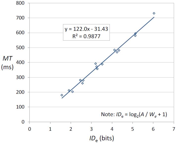
Table 17.1 includes an additional column for the effective target width (We), computed using the discrete-error method. A re-analysis of the data in Table 17.1 using We and the Shannon formulation for the index of difficulty is shown in Figure 17.5. The fit of the model is improved (R2 = .9877) as the data points are now closer to the best-fitting line. The curving away from the regression line for easy tasks appears corrected. Note that the range of IDs is narrower using adjusted measures (cf. Figure 17.2 & Figure 17.5). This is due to the 1-bit decrease when ID is greater than about 2 bits (see Figure 17.3) and the general increase in ID for "easy" tasks because of the narrow distribution of hits.
Figure 17.5. Re-analysis of data in Table 17.1 using the effective target width (We) and the Shannon formulation of index of difficulty (IDe).
Although Fitts' apparatus only recorded "hit" or "miss", modern computer-based systems are usually capable of recording the coordinate of target selection. (There are exceptions. Interaction methods that employ dwell-time selection perform target selection by maintaining the cursor within the target for a prescribed time interval. There is no selection coordinate per se. Examples of dwell-time selection include input using an eye tracker, such as MacKenzie, 2012 and Zhang & MacKenzie, 2007, or tilt-based input, such as Constantin & MacKenzie, 2014 and MacKenzie & Teather, 2012.)
As noted earlier, these data allow use of the standard-deviation method to calculate We. It is also possible, therefore, to calculate an effective amplitude (Ae) – the actual distance moved. The use of the Ae has little influence provided selections are distributed about the center of the targets. However, it is important to use Ae to prevent "gaming the system." For example, if all movements fall short and only traverse, say, ¾ × A, TPe is artificially inflated if calculated using A. Using Ae prevents this. This is part of the overall premise in using "effective" values: Participants get credit for what they actually did, not for what they were asked to do.
What is Fitts' Law?
At this juncture, it is worth stepping back and considering the big picture: What is Fitts' law? Among the refinements to Fitts' index of difficulty noted earlier, only the Welford and Shannon formulations were presented. Although other formulations exist, they are not reviewed here. There is a reason. In most cases, alternative formulations were introduced following a straight-forward process: A change was proposed and rationalized and then a new prediction equation was presented and empirically tested for goodness of fit. Researchers often approach this exercise in a rather single-minded way. The goal is to improve the fit. A higher correlation is deemed evidence that the change improves the model – period. But, there is a problem. The altered model often lacks any term with units "bits". And so, the information metaphor is lost. This can occur for a variety of reasons, such as using a non-log form of ID (e.g., power, linear), inserting new terms, or splitting the log-term into separate terms for A and W. If there is no term with units "bits", there is no throughput. While such models may indeed be valid, characterizing them as improvements to Fitts' law, or even as variations on Fitts' law is, arguably, wrong. They are entirely different models.
The positon taken in the above paragraph follows from two points. First, the prediction form of Fitts' law (Eq. 17.4) does not appear in Fitts' original 1954 publication. Thus, it is questionable whether any effort motivated simply to improve the fit of the prediction equation falls within the realm of Fitts' law research. Second, Fitts' law is fundamentally about the information capacity of the human motor system. (The title of Fitts' 1954 paper begins with the words set in italics.) The true embodiment of Fitts' law is Eq. 17.3 for throughput, which appears in the original paper, albeit with different labels (Fitts, 1954, Eq. 2). Thus, retaining the information metaphor is central to Fitts' law.
ISO 9241-9
In the decades after the first publication (Fitts, 1954), numerous Fitts' law studies appeared – and in a great variety of forms. While the internal validity of these studies is not in question, there is considerable inconsistency in this body of research, and this renders across-study comparisons a daunting task. Simply put, it is often not possible to compare throughput values from one study to another. Reading carefully, details are often inadequately given. Where details are given, it is clear that throughput was often calculated in different ways. Furthermore, inconsistencies exist in the data collected or in the way the data are put to work in building Fitts' law models or calculating throughput. Clearly, Fitts' law research could benefit from a standardized methodology. This is particularly true in HCI, where the practical benefits of new ideas must be assessed and compared with related ideas in other publications. Enter ISO 9241-9.
ISO standards are written by technical committees drawn from the research and applied research communities. One standard relevant to HCI is the multi-part ISO 9241, "Ergonomic requirements for office work with visual display terminals (VDTs)." Draft versions began to appear in the 1990s. Part 9 is "Requirements for non-keyboard input devices" (ISO, 2000). The standard has since been updated to the more generic title "Ergonomics of human-system interaction". The parts have also been updated, renamed, and renumbered. Part 9 is now Part 411, "Evaluation methods for the design of physical input devices" (ISO, 2012). (References in this chapter to ISO 9241-9 also apply to ISO 9241-411. With respect to the Fitts' law testing procedures, the two versions are the same.) The standard is relevant to virtually any input mechanism that can perform point-select operations on a computer. If there is one key benefit of ISO 9241-9, it is the standardization brought to the application of Fitts' law to input research in HCI.
The two main performance testing procedures in ISO 9241-9 employ the Fitts' paradigm. There is a one-dimensional (1D) task and a two-dimensional (2D) task, both using serial target selections. Including a 2D task is a pragmatic extension to Fitts' law to support interactions commonly found in computing systems. Although the possibility of a discrete task was described by Fitts (see Figure 17.1b herein) and is used in some Fitts' law studies, discrete tasks are not included in ISO 9241-9.
Screen snaps from the author's implementations are shown in Figure 17.6a for
FITTSTASKONE (1D) and in Figure 17.6b for
FITTSTASKTWO (2D).
(Available as free downloads at http://www.yorku.ca/mack/FittsLawSoftware/.
The downloads include Java source and class files, executable JAR files,
examples, and detailed APIs.)
For the 2D image,
dashed lines are superimposed to show the sequence of target selections. As
each target is selected, the highlight moves to a position across the layout
circle to reveal the next target to the participant. Figure 17.6c shows a typical
popup dialog after a sequence of trials using a mouse with
FITTSTASKTWO. The
throughput value of 4.9 bits/s is typical for a mouse in this context.
(a)(b)
(c)
Figure 17.6. Implementations of the (a) one-dimensional (FITTSTASKONE) and (b) two-dimensional (FITTSTASKTWO) tasks in ISO 9241-9. (c) Popup dialog after a sequence of trials.
ISO 9241-9 and the Fitts' paradigm have been used in many studies over the past 15 or so years. Examples of novel interactions or devices evaluated according to the standard include a trackball game controller (Natapov, Castellucci, & MacKenzie, 2009), smartphone touch input (MacKenzie, 2015), tabletop touch input (Sasangohar, MacKenzie, & Scott, 2009), Wiimote gun attachments (McArthur, Castellucci, & MacKenzie, 2009), eye tracking (Zhang & MacKenzie, 2007), glove input (Calvo, Burnett, Finomore, & Perugini, 2012), and lip input (José & de Deus Lopes, 2015). Throughput values range from about 1 bit/s for lip input to about 7 bits/s for touch input. Mouse values are typically in the 4-5 bits/s range.
Calculation of Throughput
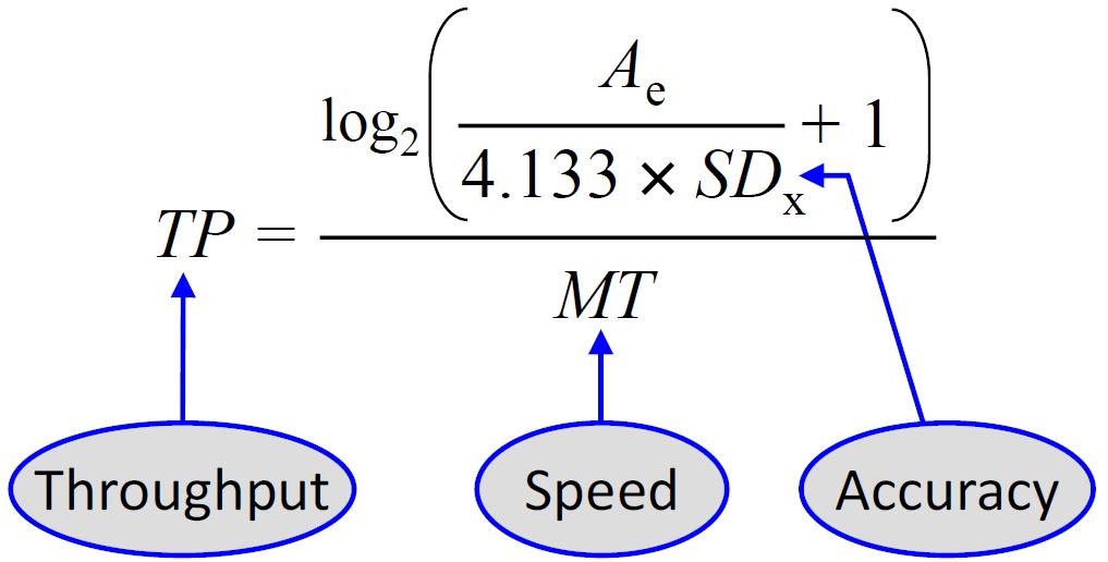
Although ISO 9241-9 provides the correct formula for Fitts' throughput, little guidance is offered on the data collection, data aggregation, or in performing the adjustment for accuracy. The latter presents a particular challenge when using the 2D task. In this section we examine the best-practice method for calculating Fitts' throughput. We begin with Figure 17.7 which shows the formula for throughput, expanded to reveal the Shannon formulation for ID and the use of effective values for target amplitude and target width. The figure also highlights the presence of speed (1 / MT) and accuracy (SDx) in the calculation.
Figure 17.7. Formula for throughput showing the Shannon formulation for ID and the adjustment for accuracy. Speed (1 / MT) and accuracy (SDx) are featured.
Whether using the 1D or the 2D task, the calculation of throughput requires Cartesian coordinate data for each trial. Data are required for three points: the starting position ("from"), the target position ("to"), and the trial-end position ("select"). See Figure 17.8. Although the figure shows a trial with horizontal movement to the right, the calculations described next are valid for movements in any direction or angle. Circular targets are shown to provide a conceptual visualization of the task. Other target shapes are possible, depending on the setup in the experiment.
Figure 17.8. Geometry for a trial.
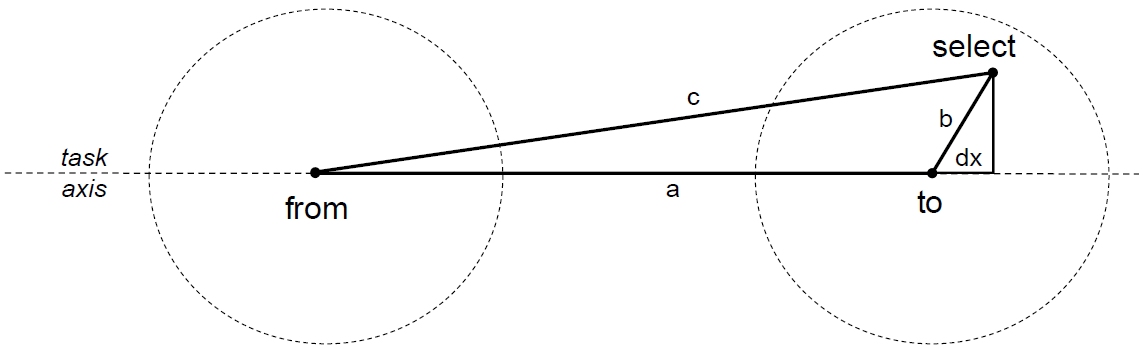
The calculation begins by computing the length of the sides connecting the
from, to, and select points in the figure. Using Java syntax,
double a = Math.hypot(x1 - x2, y1 - y2); double b = Math.hypot(x - x2, y - y2); double c = Math.hypot(x1 - x, y1 - y);
The x-y coordinates correspond to the from (x1, y1),
to (x2, y2), and select
(x, y) points in the figure. Given a, b, and c, as above,
dx and ae are then
calculated:
double dx = (c * c − b * b − a * a) / (2.0 * a); double ae = a + dx;
Note that dx is 0 for a selection at the center of the target (as projected on
the task axis), positive for a selection on the far side of center, and
negative for a selection on the near side. It is an expected behaviour that
some selections will miss the target.
The effective target amplitude (Ae) is ae in the code above. It is the actual
point-to-point movement distance for the trial, as projected on the task axis.
For serial responses, an additional adjustment for Ae is to add dx from the
previous trial (for all trials after the first). This is necessary since each
trial begins at the selection point of the previous trial. For discrete
responses, each trial begins at the center of the from target.
Given arrays for the from, to, and select points in a sequence of trials and
the computed ae and dx for each trial, Ae is the mean of the ae values and
SDx
is the standard deviation in the dx values. With these, TPe is computed using
Eq. 17.6 (substituting Ae and We = 4.133 × SDx) and throughput (TP) is
computed using Eq. 17.3 (using IDe). See also the equation in Figure 17.7. Of
course, movement time (MT) is the mean of the times recorded for all trials in
the sequence.
One final point concerns the unit of analysis for calculating throughput. The correct unit of analysis for throughput is an un-interrupted sequence of trials for a single participant. The premise for this is twofold:
- Throughput cannot be calculated on a single trial;
- A sequence of trials is the smallest unit of action for which throughput can
be attributed as a measure of performance.
The second point is of ecological concern. After a sequence of trials, the participant pauses, stretches, adjusts the apparatus, has a sip of tea, adjusts her position on a chair, or something. There is a demarcation between sequences and for no particular purpose other than to provide a break or pause, or perhaps to change to a different test condition. It is reasonable to assert that once a sequence is over, it is over! Behaviours were exhibited, observed, and measured and the next sequence is treated as a separate unit of action with separate performance measurements.
Given the above points, a closer look at the calculation of throughput is warranted. Consider Table 17.1. Each row in the table summarizes the results for 16 participants performing two 15-second sequences of trials at the indicated A and W. For each sequence, MT = 15 / m, where m is the number of stylus taps. MT in the table is the mean computed over 16 participants, two sequences each. ID in the table is calculated from A and W using Eq. 17.2. Throughput for each row is calculated once, as ID / MT from the values in that row. The expanded formula for TP is as follows:
|
| (17.7) |
where n is the number of Participant × Sequence combinations – 32 in this case. But, the correct calculation, respecting the appropriate unit of analysis, is
|
| (17.8) |
With Eq. 17.8, throughput is calculated on each sequence of trials. The overall throughput is the mean of n values. Eq. 17.7 and Eq. 17.8 will yield the same value for the data in Table 17.1, because the iterated values for ID are the same across participants and sequences. But, when Crossman's adjustment for accuracy is used, the situation is different. The numerator in Eq. 17.7 is IDe computed using We, as described earlier. Spatial variability is distilled into a single value which in turn spawns a single IDe. Let's call this ID'e. Eq. 17.7, with the adjustment for accuracy, is then
|
| (17.9) |
In essence, the accuracy component in a sequence of trials is differed. Accuracy is included at the end as a single composite adjustment applicable to all participants and trial sequences. Given the complexity of the log-term for ID, this method is likely to introduce a bias in the calculation of throughput. Again, respecting the unit of analysis, the correct calculation for throughput including the adjustment for accuracy is
|
| (17.10) |
Eq. 17.10 treats each sequence of trials as a separate unit of action. Speed and accuracy come together into a single measure of participant behaviour, throughput. These measures are then summed and averaged across participants and trial sequences.
Eq. 17.9 and Eq. 17.10 will yield different values for throughput. For the data in Table 17.1, TP = 8.97 bits/s using Eq. 17.9. This is in contrast to the value of TP = 10.10 bits/s seen in Table 17.1, which uses Eq. 17.7. It is not possible to recalculate throughput using Eq. 17.10 because the data from Fitts' experiment are not available for each participant on each trial sequence.
In summary, reducing the data from a Fitts' law experiment as in Table 17.1, while useful for summarizing participant responses or building a Fitts' law prediction equation (see Eq. 17.4), is not recommended if the goal is to measure the rate of information transfer (i.e., throughput; see Eq. 17.3 and Figure 17.7). For this, Eq. 17.10 should be used with each value for IDe computed using Eq. 17.3 (as per Figure 17.7) on the data from a single sequence of trials. Here again we see a distinction between Fitts' law as a model for predicting and Fitts' law as a model for measuring. Let's continue with an example of the use of Fitts' throughput for interactions typically found in contemporary computing systems.
Example User Study
We now put together the ideas above in an example user study investigating touch-based target selection on a smart phone.2 Since 1D and 2D task types are both common in Fitts' law studies, it is worth asking whether there is an inherent difference in throughput for a 1D task compared to a 2D task. It seems this question has not been explored in a systematic way, that is, using task type (1D vs. 2D) as an independent variable in a controlled experiment.
Participants
Participants were recruited from the local university campus. The only stipulation was that participants were regular users of a touchscreen phone, pad, or tablet. Sixteen participants were recruited from a wide range for disciplines. Six were female. The mean age was 24.3 years (SD = 3.0). Participants' average touchscreen experience was 22.9 months (SD = 15.8). All participants were right-handed.
Apparatus (Hardware and Software)
The testing device was an LG Nexus 4 touchscreen smartphone running Android OS version 4.2.2. The display was 61 × 102 mm (2.4 in × 4.0 in) with a resolution of 768 × 1184 pixels and a pixel density of 320 dpi. All communication with the phone was disabled during testing.
Custom Android software called FITTSTOUCH was developed using Java SDK 1.6. The software implemented the serial 1D and 2D tasks commonly used in Fitts' law experiments and prescribed in ISO 9241-9. (FITTSTOUCH is available as a free download including source code. See above.)
The same target amplitude and width conditions were used for both task types. The range was limited due to the small display and finger input. In all, six combinations were used: A = { 156, 312, 624 } pixels × W = { 78, 130 } pixels. These corresponded to task difficulties from ID = 1.14 bits to ID = 3.17 bits (see Eq. 17.6). A wider range is desirable but pilot testing revealed very high error rates for smaller targets. (This due to a phenomenon of touch input known as the fat-finger problem – Wigdor, Forlines, Baudisch, Barnwell, & Shen, 2007.) The scale of target conditions was chosen such that the widest condition (largest A, largest W) spanned the width of the display (portrait orientation) minus 10 pixels on each side. Examples of target conditions are shown in Figure 17.9.
(a)(b)
(c)
Figure 17.9. Example task conditions. (a) 1D with A = 312 & W = 78. (b) 2D with A = 156 & W = 130. (c) 2D with A = 624 & W = 78. All units pixels.
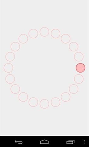
The 2D conditions included 20 targets, which was the number of trials in a sequence. The target to select was highlighted. Upon selection, the highlight moved to the opposite target. Selections proceeded in a rotating pattern around the layout circle until all targets were selected. For the 1D task, selections were back and forth. Data collection for a sequence began on the first tap and ended after 20 target selections (21 taps).
Procedure
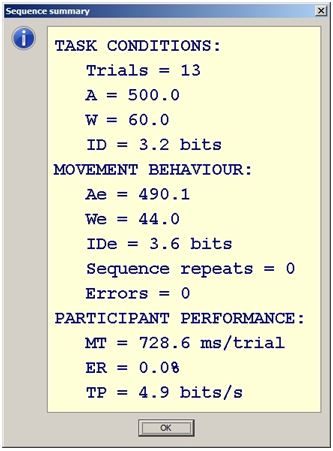
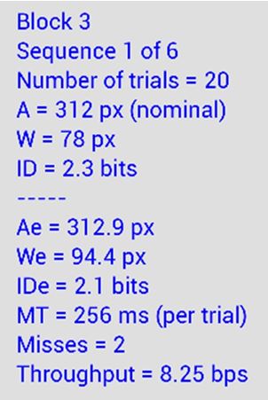
After signing a consent form, participants were briefed on the goals of the experiment. The experiment task was demonstrated to participants, after which they did a few practice sequences. They sat at a desk with the device positioned on the desk surface. They were allowed to anchor the device with their non-dominant hand, if desired. An example of a participant performing trials in the 1D condition is shown in Figure 17.10a. An auditory beep sounded if a target was missed. At the end of each sequence a dialog appeared showing summary results for the sequence. See Figure 17.10b for an example. The dialog is useful for demos and to help inform and motivate participants during testing.
(a)(b)
Figure 17.10. (a) A participant performing trials in the 1D condition. (b) Example dialog at the end of a sequence.
Participants were asked to select targets as quickly and accurately as possible, at a comfortable pace. They were told that missing an occasional target was OK, but that if many targets were missed, they should slow down.
Design
The experiment was fully within-subjects with the following independent variables and levels:
Task 1D, 2D Block 1, 2, 3, 4, 5 Amplitude 156, 312, 624 pixels Width 78, 130 pixels
The primary independent variable was task. Block, amplitude, and width were included to gather a sufficient quantity of data over a reasonable range of task difficulties.
For each condition, participants performed a sequence of 20 trials. The task conditions were counterbalanced with 8 participants per order. The amplitude and width conditions were randomized within blocks.
The dependent variable was throughput. Testing lasted about 45 minutes per participant. The total number of trials was 16 Participants × 2 Tasks × 5 Blocks × 3 Amplitudes × 2 Widths × 20 Trials = 19,200.
Results and Discussion
The grand mean for throughput was 6.85 bits/s. This result, in itself, is remarkable. Here we see empirical evidence underpinning the tremendous success of contemporary touch-based interaction. Not only is the touch experience appealing, touch performance is measurably superior compared to traditional interaction techniques. For desktop interaction the mouse is well-known to perform best for most point-select interaction tasks. (A possible exception is the stylus. Performance with a stylus is generally as good as, or sometimes slightly better than, a mouse – see MacKenzie et al., 1991.) In a review of Fitts' law studies following the ISO 9241-9 standard, throughput values for the mouse ranged from 3.7 bits/s to 4.9 bits/s (Soukoreff & MacKenzie, 2004, Table 5). The value just reported for touch input reveals a performance advantage for touch in the range of 40% to 85% compared to a mouse. (Of course, a direct comparison is not possible since mouse input is not supported on small touchscreen devices such the LG Nexus 4 used in this study.) The most likely reason lies in the distinguishing properties of direct input vs. indirect input. With a mouse or other traditional pointing device, the user manipulates a device to indirectly control an on-screen tracking symbol. Selection requires pressing a button on the device. With touch input there is neither a tracking symbol nor a button: Input is direct!
The results for throughput by participant and task are shown in Table 17.2. The 1D task yielded a throughput of 7.43 bits/s, which was 18.5% higher than the mean of 6.27 bits/s for the 2D task. The difference was statistically significant (F1,15 = 29.8, p < .0001). All participants had higher throughput for the 1D task. Throughput was fairly flat over the five blocks of testing with < 3% change in throughput from block 1 to block 5. Consequently, a breakdown of results by block is not given.
Table 17.2
Throughput (bits/s) by participant and task.
Participant Task 1D 2D P01 6.28 6.19 P02 4.83 4.79 P03 5.90 5.34 P04 7.05 5.42 P05 7.83 5.83 P06 6.72 5.65 P07 6.38 5.05 P08 7.45 6.62 P09 8.26 6.09 P10 6.42 6.40 P11 8.33 5.94 P12 9.37 8.30 P13 8.75 6.17 P14 7.26 5.88 P15 9.01 7.76 P16 8.97 8.84 Mean 7.43 6.27 SD 1.30 1.13
The higher throughput for the 1D condition is explained as follows. With side-to-side movement only, the 1D condition is easier. Movements in the 2D condition are more complicated, since the direction of movement changes by 360° / 20 = 18° with each trial. Furthermore, occlusion is unavoidable for some trials in a sequence. This does not occur for the 1D task.
Throughput was calculated using Eq. 17.3 using the Shannon formulation for ID along with Ae and We (as per Figure 17.7). The unit of analysis for the calculation was a sequence of trials, as discussed earlier. Each value of throughput in Table 17.2 is therefore the mean of 30 values of throughput, since each participant performed five sequences of trials (1 per block) for each of six A-W conditions.
Figure 17.11 shows a chart of the findings for throughput by task, as might appear in a research paper. The error bars show ±1 SD using the values along the bottom row in Table 17.2.
Figure 17.11. Throughput (bits/s) by task. Error bars show ±1 SD.

Conclusion
This chapter has provided an overview of Fitts' law in view of current practice in human-computer interaction (HCI). It is important to bear in mind the long history of Fitts' law research in other fields and in the early years of HCI. In the 1950s, when Fitts proposed his model of human movement, graphical user interfaces and computer pointing devices did not exist. Yet, throughout the history of HCI (since Card et al., 1978), research on point-select computing tasks is inseparable from Fitts' law. The initial studies focused on device comparisons and model conformity. Since then – and partly due to the publication of ISO 9241-9 – focus has shifted to the use of Fitts' throughput (in "bits/s") as a dependent variable. This is in keeping with Fitts' original intention to explore the information capacity of the human motor system. Much of this research has seen Fitts' law applied to topics only peripherally related to pointing devices. Examples include expanding targets, hidden targets, fish-eye targets, pointing on the move, eye tracking, force feedback, tilt input, gravity wells, multi-monitor displays, wearable computing, accessible computer, virtual reality, 3D, magic lenses, and so on. Research in these topics, and others, has thrived on the theory and information metaphor inspired and guided by Fitts' law. This is Fitts' legacy to research in human-computer interaction.
References
Calvo, A., Burnett, G., Finomore, V., & Perugini, S. (2012). The design, implementation, and evaluation of a pointing device for a wearable computer. Proceedings of the Human Factors and Ergonomics Society 56th Annual Meeting - HFES 2012, 521-525, Santa Monica, CA: HFES.
Card, S. K., English, W. K., & Burr, B. J. (1978). Evaluation of mouse, rate-controlled isometric joystick, step keys, and text keys for text selection on a CRT. Ergonomics, 21, 601-613.
Constantin, C., & MacKenzie, I. S. (2014). Tilt-controlled mobile games: Velocity-control vs. position-control. Proceedings of the 6th IEEE Consumer Electronics Society Games, Entertainment, Media Conference - IEEE-GEM 2014, 24-30, New York: ACM.
Crossman, E. R. F. W., & Goodeve, P. J. (1983). Feedback control of hand-movement and Fitts' law: Communication to the Experimental Society. Journal of Experimental Psychology, 35A, 251-278.
Fitts, P. M. (1954). The information capacity of the human motor system in controlling the amplitude of movement. Journal of Experimental Psychology, 47, 381-391.
Fitts, P. M., & Peterson, J. R. (1964). Information capacity of discrete motor responses. Journal of Experimental Psychology, 67, 103-112.
Fitts, P. M., & Radford, B. K. (1966). Information capacity of discrete motor responses under different cognitive sets. Journal of Experimental Psychology, 71, 475-482.
Gillan, D. J., Holden, K., Adam, S., Rudisill, M., & Magee, L. (1990). How does Fitts' law fit pointing and dragging? Proceedings of the ACM SIGCHI Conference on Human Factors in Computing Systems - CHI '90, 227-234, New York: ACM.
Goldman, S. (1953). Information Theory. New York. Prentice-Hall.
Hick, W. E. (1952). On the rate of gain of information. Quarterly Journal of Experimental Psychology, 4, 11-36.
Hyman, R. (1953). Stimulus information as a determinant of reaction time. Journal of Experimental Psychology, 45, 188-196.
ISO. (2000). Ergonomic requirements for office work with visual display terminals (VDTs) - Part 9: Requirements for non-keyboard input devices (ISO 9241-9): International Organisation for Standardisation.
ISO. (2012). Evaluation methods for the design of physical input devices - ISO/TC 9241-411: 2012(E): International Organisation for Standardisation.
José, M. A., & de Deus Lopes, R. (2015). Human-computer interface controlled by the lip. IEEE Journal of Biomedical and Health Informatics, 19(1), 302-308.
MacKenzie, I. S. (1989). A note on the information-theoretic basis for Fitts' law. Journal of Motor Behavior, 21, 323-330.
MacKenzie, I. S. (1991). Fitts' law as a performance model in human-computer interaction. (Doctoral Dissertation), University of Toronto (http://www.yorku.ca/mack/phd.html).
MacKenzie, I. S. (1992). Fitts' law as a research and design tool in human-computer interaction. Human-Computer Interaction, 7, 91-139.
MacKenzie, I. S. (2012). Evaluating eye tracking systems for computer input. In P. Majaranta, H. Aoki, M. Donegan, D. W. Hansen, J. P. Hansen, A. Hyrskykari & K.-J. Räihä (Eds.), Gaze interaction and applications of eye tracking: Advances in assistive technologies (pp. 205-225): Hershey, PA: IGI Global.
MacKenzie, I. S. (2013). A note on the validity of the Shannon formulation for Fitts' index of difficulty. Open Journal of Applied Science, 3(6), 360-368.
MacKenzie, I. S. (2015). Fitts' throughput and the remarkable case of touch-based target selection. Proceedings of HCI International - HCII 2015 (LNCS 9170), 238-249, Switzerland: Springer.
MacKenzie, I. S., Sellen, A., & Buxton, W. (1991). A comparison of input devices in elemental pointing and dragging tasks. Proceedings of the ACM SIGCHI Conference on Human Factors in Computing Systems - CHI '91, 161-166, New York: ACM.
MacKenzie, I. S., & Soukoreff, R. W. (2003). Card, English, and Burr (1978) - 25 years later. Extended Abstracts of the ACM SIGCHI Conference on Human Factors in Computing Systems - CHI 2003, 760-761, New York: ACM.
MacKenzie, I. S., & Teather, R. J. (2012). FittsTilt: The application of Fitts' law to tilt-based interaction. Proceedings of the 7th Nordic Conference on Human-Computer Interaction - NordiCHI 2012, 568-577, New York: ACM.
McArthur, V., Castellucci, S. J., & MacKenzie, I. S. (2009). An empirical comparison of "Wiimode" gun attachments for pointing tasks. Proceedings of the ACM Symposium on Engineering Interactive Computing Systems – EICS 2009, 203-208, New York: ACM.
Meyer, D. E., Abrams, R. A., Kornblum, S., Wright, C. E., & Smith, J. E. K. (1988). Optimality in human motor performance: Ideal control of rapid aimed movements. Psychological Review, 95, 340-370.
Natapov, D., Castellucci, S. J., & MacKenzie, I. S. (2009). ISO 9241-9 evaluation of video game controllers. Proceedings of Graphics Interface 2009, 223-230, Toronto: CIPS.
Reza, F. M. (1961). An Introduction to Information Theory. New York. McGraw-Hill.
Sasangohar, F., MacKenzie, I. S., & Scott, S. (2009). Evaluation of mouse and touch input for a tabletop display using Fitts' reciprocal tapping task. Proceedings of the 53rd Annual Meeting of the Human Factors and Ergonomics Society - HFES 2009, 839-843, Santa Monica, CA: HFES.
Shannon, C. E., & Weaver, W. (1949). The mathematical theory of communications. Urbana, Il. Urbana, IL: University of Illinois Press.
Soukoreff, R. W., & MacKenzie, I. S. (2004). Towards a standard for pointing device evaluation: Perspectives on 27 years of Fitts' law research in HCI. International Journal of Human-Computer Studies, 61, 751-789.
Ware, C., & Mikaelian, H. H. (1987). An evaluation of an eye tracker as a device for computer input. Proceedings of the CHI+GI '87 Conference on Human Factors in Computing Systems and Graphics Interface, 183-188, New York: ACM.
Welford, A. T. (1960). The measurement of sensory-motor performance: Survey and reappraisal of twelve years progress. Ergonomics, 3, 189-230.
Welford, A. T. (1968). Fundamentals of skill. London. Methuen.
Wigdor, D., Forlines, C., Baudisch, P., Barnwell, J., & Shen, C. (2007). Lucid touch: A see-through mobile device. Proceedings of the ACM Symposium on User Interface Software and Technology - UIST 2007, 269-278, New York: ACM.
Zhang, X., & MacKenzie, I. S. (2007). Evaluating eye tracking with ISO 9241 -- Part 9. Proceedings of HCI International 2007, 779-788, Heidelberg: Springer.
-----
Footnotes:
1. Since the early 1990s, use of the effective target width has increased, particularly in human-computer interaction. This is in part due to the recommended use of We in the performance evaluations described in ISO 9241-9 (ISO, 2000). The first use of We in HCI is the Fitts' law study described by MacKenzie, Sellen, and Buxton (1991).
2. The example is a subset of a larger user study (see MacKenzie, 2015). The full study included an additional independent variable (device position: supported vs. mobile) and additional dependent variables (movement time, error rate). The original study also examined results by participant finger size and tested the distribution characteristics of selection coordinates. Consult for details.