2. DETAILED ANALYSIS
The theoretical issues presented and tested in this research are developed in this chapter. We begin with an analysis of Fitts' original experiments and then explore ways in which the model can be applied to computer input tasks. Along the way, research questions are posed that underlie the present investigation. These are re-stated later in more formal terms as a prelude to the three experiments.
2.1 The Original Experiments
Fitts' original investigation (1954) involved four experiments: two reciprocal tapping tasks (1-oz stylus and 1-lb stylus), a disc transfer task, and a pin transfer task. In the tapping experiments the subjects moved a stylus back and forth between two metal bars as quickly as possible and tapped the bars at their centres (see Figure 1). This experimental arrangement is commonly called the "Fitts' paradigm".
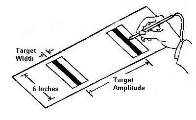
Figure 1. The reciprocal tapping paradigm (after Fitts, 1954)
Since summary data were published in Fitts' original report, and because this body of work is so vital to our investigation, the tapping experiments will be analysed in detail to develop (and correct) some of the concepts in the information processing analogy. Table 1 reproduces the data from the 1-oz tapping experiment with one column of additional data that will be discussed shortly.
Data from Fitts' (1954) Tapping Task Experiment with 1-oz Stylus
| A (in.) | W (in.) | We(DE) a (in.) | ID (bits) | MT (ms) | Errors (%) | IP b (bits/s) |
|---|---|---|---|---|---|---|
| 2 | 2.00 | 1.020 | 1 | 180 | 0.00 | 5.56 |
| 2 | 1.00 | 0.725 | 2 | 212 | 0.44 | 9.43 |
| 4 | 2.00 | 1.233 | 2 | 203 | 0.08 | 9.85 |
| 2 | 0.50 | 0.444 | 3 | 281 | 1.99 | 10.68 |
| 4 | 1.00 | 0.812 | 3 | 260 | 1.09 | 11.54 |
| 8 | 2.00 | 1.576 | 3 | 279 | 0.87 | 10.75 |
| 2 | 0.25 | 0.243 | 4 | 392 | 3.35 | 10.20 |
| 4 | 0.50 | 0.468 | 4 | 372 | 2.72 | 10.75 |
| 8 | 1.00 | 0.914 | 4 | 357 | 2.38 | 11.20 |
| 16 | 2.00 | 1.519 | 4 | 388 | 0.65 | 10.31 |
| 4 | 0.25 | 0.244 | 5 | 484 | 3.41 | 10.33 |
| 8 | 0.50 | 0.446 | 5 | 469 | 2.05 | 10.66 |
| 16 | 1.00 | 0.832 | 5 | 481 | 1.30 | 10.40 |
| 8 | 0.25 | 0.235 | 6 | 580 | 2.78 | 10.34 |
| 16 | 0.50 | 0.468 | 6 | 595 | 2.73 | 10.08 |
| 16 | 0.25 | 0.247 | 7 | 731 | 3.65 | 9.58 |
| Mean | 392 | 1.84 | 10.10 | |||
| SD | 157 | 1.22 | 1.33 | |||
|
a data added (see text) b IP = ID / MT | ||||||
As evident, target width and target amplitude varied across four levels resulting in IDs of 1 to 7 bits. Mean movement time ranged from 180 ms to 731 ms with each score derived from over 600 observations. Fitts calculated IP directly by dividing ID by MT (see Equation 2). A quick glance at the table shows the strong evidence for Fitts' thesis that the rate of information processing is constant across a range of task difficulties. The mean value of IP = 10.10 bits/s (SD = 1.33 bits/s) is purportedly the information processing rate of the human motor system for this task.
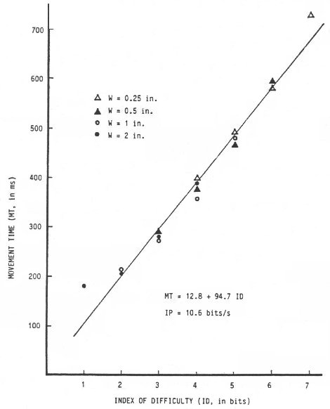
Correlating MT with ID yields r = .9831 (p = .001). It is noteworthy of the model in general that correlations above .9000 consistently emerge. Regressing MT on ID yields the following prediction equation for movement time (ms):
| MT = 12.8 + 94.7 ID. | (7) |
Calculating IP from the reciprocal of the slope yields an information processing rate of 10.6 bits/s. This rate is slightly higher than that obtained through direct calculation since it is derived from a least-squares regression equation with a positive intercept. When IP is calculated directly, the linear relationship is given an intercept of zero. A positive intercept reduces the slope of the line, thus increasing IP. Although some researchers cite values of IP calculated directly (notably Fitts, 1954), most use the statistical technique of linear regression and provide a value for IP (the reciprocal of the slope) and an intercept.
2.2 Problems Emerge
Despite the high correlation between ID and the observed mean movement time, problems with the model have been noted. A scatter plot reveals an upward curvature of movement time away from the regression line for IDs of 1 and 2 bits (see Figure 2). This systematic departure of observations from predictions was first pointed out by Crossman in 1957 (Welford, 1960) and has appeared in other studies since (Buck, 1986; Epps, 1986; Crossman & Goodeve, 1983; Drury, 1975; Klapp, 1975; Langolf, Chaffin, & Foulke, 1976; Meyer, Abrams, Kornblum, Wright, & Smith, 1988; Wallace, Newell, & Wade, 1978).
Figure 2. Scatter plot of movement time vs. index of difficulty using data from Fitts' (1954) 1-oz tapping experiment
The failure of the model when ID is small is also evident in Table 1. The index of performance rating of 5.56 bits/s when ID = 1 bit is over 3 standard deviations from the mean value of 10.10 bits/s.
Another problem stems from the relative contributions of A and W in the prediction equation. By Equation 6, the contributions should be equal, but inverse. Doubling the target amplitude adds 1 bit to the index of difficulty and increases the predicted movement time. The same effect is predicted from Equation 6 if target width is halved. In a detailed analysis of Fitts' (1954) four experiments, M. R. Sheridan (1979) showed that reductions in target width disproportionately increase movement time compared to similar increases in target amplitude. Others have also independently pointed out this disparity (Keele, 1973, p. 112; Meyer et al., 1988, p. 354; Welford, Norris, & Shock, 1969). It is also evident in scatter plots in some reports, although not noted by the investigators (Buck, 1986; Jagacinski & Monk, 1985; Jagacinski, Repperger, Ward, & Moran, 1980).
An error rate analysis may also reveal the inequitable contributions of A and W. Wade, Newell, and Wallace (1978) found a significant main effect between error rate and target width (F2,40 = 16.60, p < .01) with errors increasing as target width decreased, but no main effect between error rate and target amplitude. A similar observation was made by Card et al. (1978).
2.3 Variations of Fitts' Law
In an effort to improve the data-to-model fit, numerous researchers have proposed variations on Fitts' relationship or have introduced new models derived from different principles. Welford's (1960) variation is the most widely accepted and commonly appears in two forms:
| MT = a + b log2( (A + 0.5 W) / W) |
or
| MT = a + b log2(A / W + 0.5). | (8) |
Many researchers, including Fitts, have reported higher MT-ID correlations using Welford's formulation (Beggs, Graham, Monk, Shaw, & Howarth, 1972; Drury, 1975; Fitts & Peterson, 1964; B. A. Kerr & Langolf, 1977; Knight & Dagnall, 1967; Kv:lseth, 1980). Although Fitts' original formulation (Equation 6) is still the most frequently used, many researchers (most notably in the present context, Card et al., 1978) prefer Equation 8.
Recently it was shown that Fitts derived his relationship from an approximation of Shannon's theorem which was originally introduced with the caution that it is useful only if the signal-to-noise ratio is large (Fitts, 1954, p. 388; Goldman, 1953, p. 157; MacKenzie, 1989). The signal-to-noise ratio in Shannon's theorem corresponds to the ratio of target amplitude to target width in Fitts' analogy. As evident in Table 1, Fitts' experiments employed conditions with A:W ratios as low as 1:1! The variation of Fitts' law suggested by direct analogy with Shannon's information theorem is
| MT = a + b log2((A + W) / W) |
or the alternate form
| MT = a + b log2(A / W + 1). | (9) |
The difference between Equation 9 and Equation 6 (Fitts' law) is illustrated by comparing changes in the logarithm term (ID) as A approaches zero with W held constant (see Figure 3). It is noteworthy of Equation 9 that the logarithm cannot be negative. (Welford's equation produces a similar curve to Equation 9 except that ID approaches 1 bit as A approaches zero.)
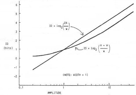
Figure 3. Index of difficulty for the Fitts and Shannon models
Obviously, a negative rating for task difficulty presents a theoretical problem. It is a minor consolation that this can only occur with Fitts' expression when the targets overlap; that is, when A < W / 2. Although such conditions may seem unreasonable, the possibility has been investigated before (Schmidt, 1988, p. 271; Welford, 1968, p. 145), and can occur when output measures are adjusted to reflect the variance in subjects' responses (using a technique we will describe shortly). Regardless, numerous researchers actually report experimental conditions with a negative ID (Card et al., 1978; Crossman & Goodeve, 1983; Gillan, Holden, Adam, Rudisill, & Magee, 1990; Ware & Mikaelian, 1987).
The practical consequences of using Equation 9 in lieu of Fitts' or Welford's equation are probably slight, and are likely to surface only in experimental settings with IDs extending under approximately 3 bits, as suggested from Figure 3. Nevertheless the theoretical implications of Equation 9 are considerable. First, the idea that similar changes in target amplitude and target width should effect a similar but inverse change in movement time, as suggested in Equation 6, does not follow in Equation 9.
Also, the sound theoretical premise for Equation 9, casts doubt on the rationale for a popular and mathematically correct variation of Fitts' formulation which separates A and W:
| MT = a + b1 log2 A + b2 log2W. | (10) |
Welford (1968, p. 156) suggests that b1log2A may correspond to an initial open-loop impulse toward a target and b2log2W may correspond to a feedback-guided final adjustment as a move terminates. Numerous researchers have used or analysed Equation 10 with good results (Bainbridge & Sanders, 1972; Gan & Hoffmann, 1988; Jagacinski, Repperger, Moran, & Glass, 1980; Jagacinski, Repperger, Ward, & Moran, 1980; Kay, 1960; R. Kerr, 1978; Sheridan, 1979; Welford, 1968; Welford et al., 1969; Zelaznik, Mone, McCabe, & Thaman, 1988). In multiple correlation analyses, it always yields a higher R than the single factor r obtained using Equation 6 (because of the extra degree of freedom); however, the model ceases to have an information-theoretic premise since similar recasting is not possible using Equation 9, which directly mimics Shannon's original theorem. For example, in Equation 10, what is ID? What is IP?
Research Question: Does Fitts' model (Equation 6) account for observations as well as Welford's model (Equation 8) or a model based directly on Shannon's information theorem (Equation 9)? (H1)
2.4 Effective Target Width
Of greater practical importance is a technique to adjust output measures to bring the model in line with the underlying principles. The technique calls for target width to be adjusted to reflect what a subject actually did (output condition), rather than what a subject was expected to do (input condition). Thus, at the model building stage, W is a dependent variable rather than an independent variable.
The output or "effective" target width (We) is derived from the observed distribution of "hits", as described by Crossman and Welford (see Welford, 1968, pp. 147-148). This adjustment lies at the very heart of the information- theoretic metaphor — that movement amplitudes are analogous to "signals" and end-point variability (viz., target width) is analogous to "noise". In fact, the information theorem upon which Fitts' law is based — particularly as expressed in Equation 9 — is built on the premise that the signal is "perturbed by white thermal noise" (Shannon & Weaver, 1949, p. 100). The analogous requirement for motor tasks is a Gaussian or normal distribution of spatial coordinates. This property has been observed in output tasks (Crossman & Goodeve, 1983; Fitts, 1954; Fitts & Radford, 1966; Welford, 1968, p. 154; Welford et al., 1969; Woodworth, 1899).
The experimental implication of normalizing output measures is illustrated as follows. The entropy (H), or information, in a normal distribution is H = log2(( 2 π e)½ × σ) = log2(4.133 × σ), where σ is the standard deviation in the unit of measurement. Splitting the constant 4.133 into a pair of z-scores for the unit-normal curve (i.e., σ = 1), we find that the area bounded by z = ±2.066 represents about 96% of the total area of the distribution. In other words, a condition that target width is analogous to the information-theoretic concept of noise is that 96% of the hits are within the target and 4% of the hits miss the target (see Figure 4a). When an error rate other than 4% is observed, target width should be adjusted to form the effective target width in keeping with the underlying theory. This is an important point that we now dwell on in more detail.
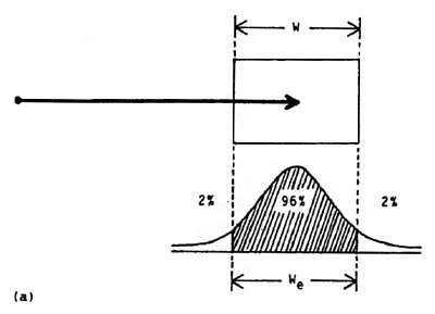
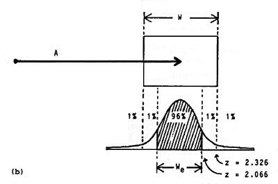
Figure 4. The method for adjusting target width
There are two methods for determining the effective target width: the standard deviation or the discrete error method. If the standard deviation in the end-point coordinates is known, just multiply SD by 4.133 to get We(SD). When the percent discrete errors is known, the method is trickier and requires a table of z-scores for areas under the unit-normal curve. Here's the method: If n percent errors are observed, find z such that ± z contains (100 − n) percent of the area under the unit-normal curve. Multiply W by 2.066 / z to get We(DE). For example, if 2% errors were recorded on a block of trials when tapping or selecting a 5 cm wide target, then We(DE) = (2.066 / z) × W = (2.066 / 2.326) × 5 = 4.45 cm (see Figure 4b).
Analyses using the effective target width should find the variation in IP reduced since, typically, subjects that take longer are more accurate and demonstrate less end-point variability. Reduced variability decreases the effective target width and therefore increases the "effective index of difficulty" (see Equation 3). On the whole, an increase in movement time is compensated for by an increase in the effective ID, and this tends to lessen the variability in IP (see Equation 2).
The technique described by Welford is not new; yet it has been largely ignored in the published body of Fitts' law research that could have benefited from it. There are several possible reasons. First, the method is tricky and its derivation from information-theoretic principles is complicated (e.g., see Reza, 1961, pp. 278-282). Second, the method is either arduous or prone to errors. Each end-point coordinate must be recorded and the standard deviation calculated over each block of trials. This is feasible using a computer for data acquisition and statistical software for analysis, but manual measurement and data entry are extremely cumbersome. Despite this, the standard deviation method is better. Recording each selection coordinate permits more behavioural patterns to be discerned, such as the predominance of overshoots vs. undershoots or the presence of outliers.
Inaccuracy occurs in the method when adjustments are based on percentage errors because the extreme tails of the unit-normal distribution are used. z scores with at least three decimal places of accuracy are needed for the factoring ratio (which is multiplied by W to get We(DE)). Manual "look-up" methods are prone to precision errors. Furthermore, "easy" conditions may have error rates too low to reveal the true distribution of hits. For example, in Table 1 Fitts reported "0.00%" errors with A = W = 2 inches, which seems reasonable since the target edges were touching. Such a condition requires a large adjustment since the distribution is very narrow (in comparison to the target width over which the hits should have been distributed – with 4% errors!). A pragmatic approach in this case is to assume an error rate of 0.0049% (which rounds to "0.00%") at worst and proceed to make the adjustment.
Introducing a post hoc adjustment on target width before the regression analysis (or maintaining a consistent error rate of around 4%) is important to maintain the information-theoretic analogy. There is a tacit assumption in Fitts' law that subjects, although instructed to move "as quickly and accurately as possible", balance the demands of tasks to meet the spatial constraint that 96% of the hits fall within the target. When this condition is not met, an adjustment to target width should be introduced. Furthermore, if subjects slow down and place undue emphasis on accuracy, the task changes; the constraints become temporal and the prediction power of the model falls off (Meyer et al., 1988). In summary, Fitts' law is a model for rapid, aimed movements and the presence of a nominal yet consistent error rate in subjects' behaviour is assumed, and arguably vital.
Research Question: Does the prediction power of the model improve by substituting for target width a measure of subjects' response variability in spatial coordinates? (H2)
2.5 Re-analysis of Fitts' Data
The technique for adjusting target width (using the discrete error method) was applied to the data in Fitts' tapping experiments to determine the effective target width. The adjusted values, We(DE), appear in Table 1 for the 1-oz tapping experiment. The correlation between ID and MT for the first experiment using Fitts' model without the adjustments is high (r = .9831, p < 001), as previously noted, but higher when ID is recalculated using We(DE) (r = .9907, p < .001) and even higher when using We(DE) and the logarithm term in Equation 9 (r = .9931, p < .001). As indicated in Table 2 the trend is similar for the other experiments.
Re-analysis of Data from Fitts' (1954) Tapping Task Experiment
| Model | Equation | Target Width | r a | Regression Coefficients | ||||
|---|---|---|---|---|---|---|---|---|
| Intercept, a (ms) | SE b | Slope, b (ms/bit) | SE b | IP (bits/s) c | ||||
| *** 1 oz Stylus *** | ||||||||
| Fitts | 6 | Unadjusted (W) | .9831 | 12.8 | 20.3 | 94.7 | 4.7 | 10.6 |
| Fitts | 6 | Adjusted (We) | .9904 | -73.2 | 18.0 | 108.9 | 4.0 | 9.2 |
| Shannon | 9 | Adjusted (We) | .9937 | -31.4 | 13.4 | 122.0 | 3.6 | 8.2 |
| *** 1 lb Stylus*** | ||||||||
| Fitts | 6 | Unadjusted (W) | .9796 | -6.2 | 24.7 | 104.8 | 5.7 | 9.5 |
| Fitts | 6 | Adjusted (We) | .9882 | -118.0 | 22.8 | 124.0 | 5.1 | 8.1 |
| Shannon | 9 | Adjusted (We) | .9925 | -69.8 | 16.6 | 138.8 | 4.5 | 7.2 |
| *** Disc Transfer *** | ||||||||
| Fitts | 6 | Unadjusted (W) | .9186 | 150.0 | 74.6 | 90.4 | 10.4 | 11.1 |
| Shannon | 9 | Unadjusted (W) | .9195 | 223.0 | 66.0 | 92.6 | 10.6 | 10.8 |
| *** Pin Transfer *** | ||||||||
| Fitts | 6 | Unadjusted (W) | .9432 | 22.3 | 48.2 | 86.1 | 7.1 | 11.6 |
| Shannon | 9 | Unadjusted (W) | .9452 | 84.4 | 42.2 | 89.4 | 7.3 | 11.2 |
|
a p < .001 b standard error c IP = 1 / b | ||||||||
A scatter plot of MT vs. ID, where ID = log2(A / We + 1) from Equation 10, shows a coalescing of points about the regression line (see Figure 5). Notice also in the scatter plot that the range of IDs is less than in Figure 2. This is due to the 1-bit difference in the Shannon model when ID is greater than about 2 bits (see Figure 3), and to the general increase in ID for "easy" tasks as reflected in the narrow distribution of hits.
Figure 5. Scatter plot and regression line using We and the Shannon formulation for ID.
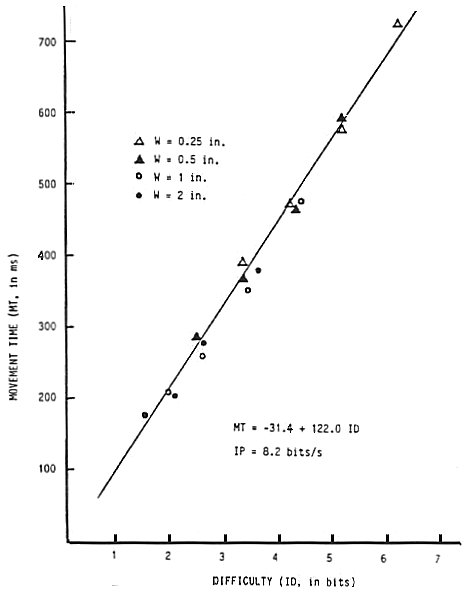
Although the regression equation obtained using Fitts' formulation is noteworthy for providing the intercept closest to the origin for all four experiments, the standard error was the highest for all four experiments. A large intercept is perhaps due the presence of factors which are unaccounted for in the experiment, such as a "button push" or other antagonistic muscle activity which occurs consistently at the beginning or end of the task (Meyer, Smith, & Wright, 1982, p. 477). In follow-up applications, a negative prediction of movement time is unlikely since task difficulties well under 1 bit would be required. The scatter plot in Figure 5 shows that the general effect of the adjustments is to increase low values of ID, and further decrease the likelihood of a negative prediction.
Note in Table 2 that IP decreases for each change introduced. Substituting We for W reduces IP because easy tasks tend to have lower error rates than hard tasks (see Table 1). Changing formulations for ID tends to reduce IP because the Shannon formulation reduces high IDs by 1 bit and slightly increases low IDs (see Figure 3). Both of these changes effect a slight counter-clockwise rotation on the points in the scatter plot which in turn increases the regression line slope and reduces IP.
Nevertheless, the magnitude of IP is of less interest to the present discussion than the overall accuracy of the model as determined by the statistical measure of correlation. Since the increased correlation using the Welford or Shannon formulation for ID was slight, a test for statistical significance in the difference should follow. Table 3 presents the results of such a test using Hotelling's t test for the difference between correlations of dependent samples (e.g., Guilford & Fruchter, 1978, p. 164). Since the Welford formulation consistently yielded correlations between those for the Fitts and Shannon formulations, only the latter two models are compared.
Test of Statistical Significance Between Models
| Experiment | Target Width | ID Range a | Correlations by Model b | Hotelling's t Test c | |||||
|---|---|---|---|---|---|---|---|---|---|
| Low | High | Fitts | Shannon | Inter-Model | t | n | p | ||
| Tapping (1 oz) | W | 1.0 | 7.0 | .9831 | .9936 | .9966 | 6.47 | 16 | .001 |
| We | 2.0 | 7.0 | .9907 | .9938 | .9988 | 2.20 | 16 | .05 | |
| Tapping (1 lb) | W | 1.0 | 7.0 | .9796 | .9916 | .9966 | 6.94 | 16 | .001 |
| We | 2.0 | 7.0 | .9885 | .9927 | .9987 | 2.83 | 16 | - | |
| Disc transfer | W | 4.0 | 10.0 | .9185 | .9195 | .9999 | 0.64 | 16 | - |
| Pin transfer | W | 3.0 | 10.0 | .9432 | .9452 | .9997 | 1.07 | 20 | - |
|
a ID computed using Fitts' formulation b p < .001 c two-tailed test, df = n − 3 | |||||||||
Several important observations follow from Table 3. First, statistical significance between the correlations appeared for the tapping experiments, with and without applying the adjustment on target width. This is good news for the Shannon model. The statistical insignificance in the differences for the disc and pin transfer experiments was perhaps due to the nature of the tasks. The tapping tasks were highly ballistic, whereas the disc and pin transfer task s were regulated by feedback mechanisms. The variations in the terminating positions for the tapping tasks were analogous to noise and were recorded as percentage errors when the subjects missed the targets. Errors, however, could not occur in the disc or pin transfer task; the subjects simply took the time necessary to guide the disc or pin until it was secured in place. The extra time spent in the final placement of the disc or pin may also explain the generally higher intercepts for those experiments (see Table 2). Another explanation, which is particularly important in distinguishing the two formulations, stems from the range of experimental conditions. As evident in the Table 3, the tapping experiments had an ID range of 1-7 bits, whereas the disc and pin transfer experiments had ID ranges of 4-10 bits and 3-10 bits respectively. It was demonstrated earlier (see Figure 3) that the difference between models is greatest for small values of ID.
Although the difference between the correlations for the tapping experiments achieved significance at the p < .001 level, the significance of the difference diminished considerably when the adjustment for effective target width was introduced. This was due to the general increase in ID for "easy" tasks because of the relatively narrow distribution of hits when the A:W ratio was small (see Figure 5). When substituting We for W, the 1-bit tasks were rated at about 2 bits.
In itself, narrowing the range of IDs tends to reduce correlations. This follows from an inherent property of correlation: When a sample is drawn from a restricted range in a population, correlations are lower than when a sample is representative of the entire population (Glass & Hopkins, 1984, p. 92). Thus, applying the technique for normalizing target width introduces two opposing influences: the tendency to improve the correlation because of the sound role of We in the model, and the tendency to reduce the correlation because the technique generally reduces the range of IDs. Furthermore, the latter influence will tend to reduce the differences between the models since low values of ID are needed for differences to appear.
To conclude, the trend of increasing correlation and decreasing standard error progressing down the columns in Table 2 for each experiment, in conjunction with the statistical significance of the improved correlations using the Shannon formulation for the tapping experiments, suggests that the adjustments introduced improve the model's accuracy.
2.6 Effective Target Amplitude
It follows from the preceding discussion that an adjustment is also in order to reflect the actual distance moved, resulting in an "effective" target amplitude, Ae. The possibility seems strongest that Ae < A, particularly when A:W is small, but many factors are at work such as the characteristics of the device employed. The data in Fitts' report do not permit an investigation of this point; however, it was observed that of the two possibilities, undershoot errors were more common (Fitts, 1954, p. 385). This trend has also been noted in other studies (Glencross & Barrett, 1983; P. A. Hancock & Newell, 1985, p. 159; Wright & Meyer, 1983).
The implications of this are subtle and may be of little practical consequence. If a prediction equation is derived using adjusted amplitude measures (reflecting what subjects actually did), and then applied in subsequent designs, there may be a systematic departure of performance from predictions. More errors may occur than predicted since output responses may not be a normally-distributed reflection of input stimulus, but may be skewed inward.
2.7 Dimensions of Movement Tasks
There are two aspects of dimensionality in Fitts' law tasks: the shape of targets and the direction of movement. When movements are limited to one dimension (e.g., back and forth) and both target height (H) and target width are varied, there is evidence that target height has only a slight main effect on movement time (Welford, 1968, p. 149; Kvalseth, 1977; Salmoni, 1983). Schmidt (1988, p. 278) and Crossman (see Welford, 1968, p. 149) note that horizontal motion toward a target results in an elliptical pattern of hits, with the long axis on the line of approach.
When the shape of the target and the direction of movement vary, the situation is confounded. For rectangular targets in 2-D positioning tasks, as the approach angle changes from 0° to 90° (relative to the horizontal axis), the roles of target width and target height reverse (see Figure 6).
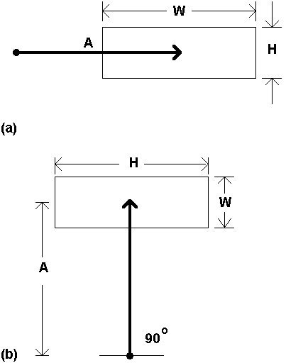
Figure 6. The changing role of target width and target height
Varying the direction of approach raises the question, "what is target width?" At the model building stage, the issue is avoided somewhat by using the effective target width (We), as described earlier. Most likely, We should be derived from the end-point variability in two-dimensions, calculated in Cartesian coordinates as (x2 + y2)½ . Although this idea awaits empirical testing, it can extend to three dimensional movements as well.
Projecting three-dimensional objects onto a two-dimensional CRT display is common on today's bit-mapped graphic systems. It follows that input strategies are needed to complete the loop and facilitate 3-D interaction. A first-order solution is to map a 2-D device into the third dimension (e.g., Chen, Mountford, & Sellen, 1988; Evans, Tanner, & Wein, 1981). Recent techniques include direct manipulation with an input glove (Foley, 1987; Tello, 1988; Zimmerman, Lanier, Blanchard, Bryson, & Harvill, 1987) or maneuvering a mouse in three dimensions (Ware & Baxter, 1989). Although no studies to date have employed Fitts' law in 3-D computer interaction tasks, a need may arise as this mode of interaction matures.
Research Question: Does the prediction power of the model improve by substituting for target width a measure of subjects' response variability in two (or three) dimensions? (H2)
2.8 Targets and Angles
When a derived model is used for prediction in two dimensional movement tasks, the problem of target width must be addressed directly: What value for W should be used in calculating ID? There are several possibilities. Considering first only rectangular targets, it is probably wrong to consistently use the horizontal extent of a target for W, because wide-and-short targets approached from above or below at close range will yield a negative ID (if Fitts' or Welford's formulation is used). This situation is common in text selection tasks where wide-and-short targets (viz., words) are the norm. Examples include the text selection experiments by Card et al. (1978) and Gillan et al. (1990). Both cited experimental conditions yielding negative IDs when wide targets (2.46 cm & 6 cm, respectively) were approached at close range (1 cm & 2 cm).
Research on alternative measures for target width is scarce, however. Possibilities include W + H, or W × H (Gillan et al., 1990). Perhaps "the smaller of W or H" is appropriate since the lesser of the two extents seems more indicative of the precision demands of the task. Another possibility is the span of the target along an approach vector through the centre. This distance, W', is shown in Figure 7. The latter idea is appealing in that circles or other shapes of targets can be accommodated, and because the one-dimensionality of the model is retained.
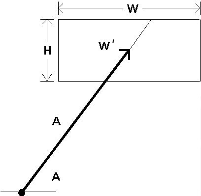
Figure 7. Incorporating approach angle in the model
As easily shown, W' can be determined using simple trigonometry. If we define θA as the angle between the approach vector and the x axis (see Figure 7), then W' is equal to H / sinθA if the approach vector intersects the top or bottom edge of the target (as shown), or W / cosθA if the approach vector intersects a side of the target.
Research Question: Does the prediction power of the model improve by re-evaluating target width in consideration of the angle of approach? (H3, H4, & H5)
2.9 Competing Models
The motivation for building models (e.g., human performance models) is that they facilitate the way we think about a problem. Models are neither right nor wrong; only through their utility do they muster support in the scientific community. Although unquestionably robust, the information processing analogy in Fitts' law does not sit well for all.
Several competing and overlapping models, including Fitts' law, are at the forefront of current research pushing toward a general theory of motor behaviour. We conclude the present chapter with a brief look beyond Fitts' law. The following paragraphs extend the belief that a general model of human movement should accommodate the extremes of temporal and spatial constraints in movement tasks. There are classes of movements (e.g., drawing) which at present lack a paradigm for performance modeling. A new model, perhaps incorporating Fitts' law, could fulfill this need.
2.9.1 The Linear Speed-Accuracy Tradeoff
Of considerable interest recently is the linear speed-accuracy tradeoff discovered by Schmidt and colleagues (Schmidt, Zelaznik, & Frank, 1978; Schmidt, Zelaznik, Hawkins, Frank, & Quinn, 1979). The tradeoff, formally the impulse variability model, forecasts that the standard deviation in end-point coordinates (viz., accuracy), is a linear function of velocity, calculated as distance over time:
| We = a + b A / MT. | (11) |
It is interesting that Equation 11 and Fitts' law contain the same three parameters (except that We is the standard deviation of end-point coordinates in Equation 11, and is 4.133 × SD in Fitts' adjusted model). Although Equation 11 can be rearranged with MT as the predicted variable, it is still fundamentally different from Fitts' law since the relationship is linear rather than logarithmic, and because the information-theoretic analogy is absent.
Another difference is the nature of the tasks suited to each. The linear speed-accuracy tradeoff is demonstrably superior to Fitts' law for "temporally constrained" tasks (Meyer et al., 1990). The distinction is summarized as follows: Under spatial constraints, a move proceeds as quickly as possible and terminates in a specified region of space (target width). This applies to Fitts' tapping task. Under temporal constraints, a move proceeds as accurately as possible and terminates after a specified time. Targets are points or lines in temporally constrained tasks. Subjects strike the target on time and avoid being too fast or too slow.
In relation to computer input, temporally constrained tasks are of a different genre. Possibilities include, for example, capturing moving targets and real-time interaction (perhaps in a music performance system). The distinction between temporal and spatial constraints is by no means dichotomous. Drawing, tracing, and inking have features of both: A user moves a tracking symbol (cursor, cross, etc.) at an optimal velocity while attending to the accuracy demands of the task. How should such tasks be modeled? Is the focus on minimizing time (the dependent variable in Fitts' law) or minimizing error (the dependent variable in Equation 11)?
The task of drawing is a simple example. The Keystroke-Level Model (Card et al., 1980) provides a rough estimate of the time to draw a series of line segments (tD in ms) from the total length of the segments (lD in cm) and the number of segments (nD). The equation
| tD = 900 nD + 160 lD | (12) |
was admittedly very restricted — dependent on the system, user, and device. It was included only to extend the generality of the Keystroke-Level Model to this class of movement tasks. Notably, accuracy is not represented in the equation. One can anticipate that a class of models for tasks with temporal constraints, such as drawing, may embody the linear speed-accuracy tradeoff given in Equation 11.
2.9.2 Power Functions
Several power functions have been proposed including the following general form (Kvalseth, 1980):
| MT = a Ab Wc | (13) |
A re-analysis of Fitts' (1954) data reveals that Equation 13 provides a higher multiple correlation (R) than the single-factor correlation (r) using Fitts' relationship. A test of positioning times using six cursor control devices also showed higher correlations using Equation 13 (Epps, 1986). Note, however, that the improved fit is largely due to the extra degree of freedom. Equation 13 has three empirically determined constants. Fitts' law has two. Furthermore, a strength of Fitts' model is the physical interpretation afforded by the terms in the equation. A similar casting is difficult for a, b, and c in Equation 13.
Several permutations of Equation 13 are possible. If b = −c, then
| MT = a (A / W)b. | (14) |
Taking the base 2 logarithm of each side yields
|
log2 MT = log2a + b
log2(A / W)
= a' + b log2(A / W) | (15) |
which is similar to Fitts' law except the log of movement time is the predicted variable (T. B. Sheridan & Ferrell, 1963).
Another permutation, introduced by Meyer et al. (1988), sets the exponent in Equation 14 to ½ and positions slope and intercept coefficients in the usual place for linear regression:
| MT = a + b (A/ W)½ | (16) |
Equation 16, formally the stochastic optimized-submovement model, is supported by a comprehensive theory on the random variability of neuromotor force pulses. In a re-analysis of Fitts' (1954) data, higher correlations were found using Equation 16 than using Fitts' law (Meyer et al., 1988); however, they are lower than those in Table 2 using the Shannon formulation.
The model provides a unified conceptual framework encompassing both the linear speed-accuracy model and Fitts' log model. Meyer and colleagues found that movements following Fitts' paradigm are composed of submovements with durations, distances, and end-point distributions conforming to the linear speed-accuracy model. This may be an important link. A goal of the stochastic optimized-submovement model is to reconcile the range of spatial and temporal demands in human movement in a general theory of motor behaviour (Meyer et al., 1990). The promise for performance modeling of user input to computers is a single model accommodating a wide range of movement tasks.