Foucault Pendulum

We program equations (6.80) from Knudsen and Hjorth ( Elements of Newtonian Mechanics , Springer 2001, 3rd ed.) in order to display the motion of the pendulum (at Paris).

The equations were derived under certain simplifying assumptions. It would be interesting to append a solution of the full equations in order to demonstrate that the approximations were justified, and also in order to have equations which are also valid for higher rotations speeds.

The latitude at Paris corresponds to sin(phi)=0.75

> restart;

> sf:=3/4;

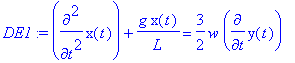
> DE1:=diff(x(t),t$2)+g/L*x(t)=2*w*sf*diff(y(t),t);

> DE2:=diff(y(t),t$2)+g/L*y(t)=-2*w*sf*diff(x(t),t);

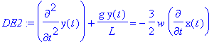
Here w is the rotation speed of the Earth, L is the pendulum arm length, and g is the gravitational acceleration.

> w:=evalf(2*Pi/(24*60*60)); # in inverse seconds

> L:=69; #69 meters

> g:=9.8;

We pick some initial conditions: an initial displacement in x , we are on the y -axis, and the pendulum bob starts with zero velocity.

> IC:=x(0)=L/10,D(x)(0)=0,y(0)=0,D(y)(0)=0;

> sol:=dsolve({DE1,DE2,IC},{x(t),y(t)});

> assign(sol);

We have a simple analytic solution for the two coupled equations!

> evalf([x(t),y(t)]);

We can plot the two components side-by-side after one half hour for about three minutes:

> plot([x(t),y(t)],t=1800..2000,color=[red,blue],thickness=3);

The initially non-existent y -component has picked up over 10 percent of the x -amplitude. Let us graph the actual trajectory at the very beginning emphasizing the beginning of the rotation (precession):

> plot([x(t),y(t),t=0..25],thickness=3);

>