Perturbation Theory

In this worksheet we provide two examples of perturbation calculations:

1) to provide a motivation for perturbative calculations we consider the first relativistic correction to the kinetic energy in the hydrogen-like ground state. It represents an example where a natural smallness parameter is present (1/c^2), and where we really are only interested in the first-order correction to the energy as the higher-order contributions do compete with corrections to the energy operator itself.

2) to show in a model problem how one can calculate higher-order corrections, and that there are examples where the series expansion is only semi-convergent we calculate the energy corrections to high, but finite order for a harmonic oscillator perturbed by a power-law (quartic) anharmonic potential. The Dalgarno-Lewis method is used to carry out the calculation.

A first-order perturbation calculation

Suppose we are interested in a calculation to account for the correction to the Schroedinger kinetic energy due to special relativity. We just consider the hydrogenic ground state which is non-degenerate.

> restart;

> assume(c>0,m>0);

> taylor(sqrt(m^2*c^4+p^2*c^2),p=0);

The rest energy in atomic units is given as

> subs(m=1,c=137,m*c^2);

> %*27.12*_eV;

This is slightly off from the accepted electron mass of 512 keV due to our approximate value of the fine structure constant as 1/137.

We know from the virial theorem that the kinetic energy in the hydrogen atom ground state has the same magnitude as the binding energy (13.6 eV). We recognize that the inverse powers of c will generate converging series. Note that in atomic units m =1.

To first order we need to calculate the expectation value of the fourth derivative for the H0-eigenstate, i.e., the hydrogenic 1s-state. The angular momentum is zero, and therefore only a radial derivative is required when considering the momentum operator as it acts on s-states.

> psi:=2*r*exp(-r);

> int(psi^2,r=0..infinity);

It is most convenient to perform the calculation in momentum space, where the momentum operator is a multiplicative operator.

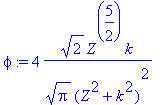
> phi:=simplify(sqrt(2/Pi)*int(psi*sin(k*r),r=0..infinity));

> int(phi^2,k=0..infinity);

If we choose units in which h_bar equals unity, we do not distinguish between p and k (momentum and wavenumber).

> int(phi^2*k^2/2,k=0..infinity);

We recognize that the non-relativistic kinetic energy is calculated correctly. Let us now obtain the

> int(phi^2*(-k^4/(8*c^2)),k=0..infinity);

> evalf(subs(c=137,%));

This is a very small correction when compared to the non-relativistic answer of 0.5. Now we repeat the calculation for arbitrary Z (hydrogen-like situation).

> assume(Z>0);

> psi:=2*Z^(3/2)*r*exp(-Z*r);

> int(psi^2,r=0..infinity);

> phi:=simplify(sqrt(2/Pi)*int(psi*sin(k*r),r=0..infinity));

> No:=int(phi^2,k=0..infinity);

> T_nr:=int(phi^2*k^2/2,k=0..infinity);

> T_r1:=int(phi^2*(-k^4/(8*c^2)),k=0..infinity);

> subs(Z=20,c=137,evalf([1*c^2,T_nr,T_r1])); # Calcium

> subs(Z=79,c=137,evalf([1*c^2,T_nr,T_r1])); # Gold

> subs(Z=92,c=137,evalf([1*c^2,T_nr,T_r1])); # Uranium

It is evident that:

a) the kinetic energy becomes comparable to the rest energy for Z approaching 100 (heavy-ion collisions allow one to explore this regime).

b) the relativistic kinetic energy becomes appreciable for moderate values of Z . The Schroedinger equation is no longer adequate.

c) there are two expansions that do come up in the present context:

(i) the expansion of the relativistic kinetic energy as a power series in p;

(ii) the energy correction from the first term in this expansion beyond the non-relativistic expression has been evaluated only in first-order PT.

It is important to distinguish the two sources of expansions. The expansion of the Hamiltonian itself has as its origin the model-like character of the approach; a proper approach to special relativity would start from a different wave equation, and would be fully compliant with the modern world after Einstein. This approach for spin-1/2 particles such as electrons was introduced by Dirac. It leads not only to an equation where the relativistic kinetic energy expression is quantized, but one finds that all the magnetic interactions resulting from the particle's spin and orbital angular momenta is automatically included. One has to include perturbatively, however corrections to the Hamiltonian that arise from interactions with the nuclear magnetic moment (hyperfine structure), and further details such as nuclear finite size effects (the nucleus is not a point particle and one should take into account at short distances the extent of the nuclear charge distribution).

The Dalgarno-Lewis method for perturbation theory

In 1955 A. Dalgarno and J.T. Lewis published a method that allows to calculate the perturbation series to high orders for non-degenerate states.

The method is explained in the classic textbook by L.I. Schiff (QM, McGraw-Hill, 3rd ed., 1968, chapter 33). The method is based on the conversion of an eigenvalue problem into a series of inhomogeneous differential equations. These equations determine successively the corrections to the eigenfunctions, and the energy corrections are obtained by a simple expectation value. For the equations read:

(H0-E[0]) psi[0] = 0

(H0-E[0]) psi[1] = (E[1]-W) psi[0]

(H0-E[0]) psi[2] = (E[1]-W) psi[1] + E[2] psi[0]

(H0-E[0]) psi[3] = (E[1]-W) psi[2] + E[2] psi[1] + E[3] psi[0]

...

Here , and a similar expansion holds for the wavefunction. The energy corrections are calculated from the expectation value E[i] = <psi[0]|W|psi[i-1]>. psi[0] has to be normalized.

The equations to be solved for psi[i] are inhomogeneous, as they are driven by a known right-hand side, namely the wavefunction correction obtained in the previous step. The method is started with the known solution psi[0], E[0], and E[1] is calculated directly. At every stage one has to calculate a new wavefunction from solving a distinct inhomogeneous problem, although the operator on the LHS remains the same. The energy correction is then obtained by a simple matrix element. This is in contrast with the usual approach where the second-order energy already involves an infinite sum. Note that the differential equations are of a structure where they can be solved by a Green's function that involves a sum over all H0 eigenstates.

In this worksheet we consider cases of power-law potentials that allow exact solutions to the Dalgarno-Lewis equations. The H0 problem is assumed to be the simple harmonic oscillator.

> restart;

> W:=x^4;

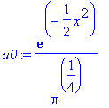
> u00:=exp(-x^2/2);

> No:=1/sqrt(int(u00^2,x=-infinity..infinity)):

> u0:=No*u00;

> E0:=1/2;

> E1:=int(u0*W*u0,x=-infinity..infinity);

Now that we have the first-order energy correction we can proceed with the calculation of the first-order wavefunction calculation:

> SE1:=-1/2*diff(f(x),x$2)+(x^2-1)/2*f(x)=u0*(E1-W);

We can solve SE1 by a matrix method. The left-hand side will be common to all subsequent equations. Inhomogeneous differential equations in matrix representations become matrix inversion problems. We use a harmonic oscillator basis for the matrix representation:

> with(orthopoly);

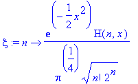
> xi:=n->exp(-x^2/2)*H(n,x)/(Pi^(1/4)*sqrt(n!*2^n));

> int(xi(4)^2,x=-infinity..infinity); # an example of normalization.

> subs(f(x)=xi(n),lhs(SE1));

> xi(m)*simplify(%);

> ME:=unapply(Int(expand(%),x=-infinity..infinity),m,n);

Now we show that the structure of the matrix is very simple indeed: only diagonal matrix elements occur, and the structure is that <n|H0-E[0]|n>=n. This diagonal matrix is trivial to invert! Check it for yourself using matrix inversion.

> value(ME(1,2));

> value(ME(2,2));

> value(ME(2,4));

> value(ME(2,6));

> value(ME(0,0));

> value(ME(4,4));

> value(ME(6,6));

> value(ME(1,1));

Error, (in GAMMA) numeric exception: division by zero

> rhs(SE1);

> RH1:=unapply(Int(expand(xi(m)*rhs(SE1)),x=-infinity..infinity),m);

The solution is given as a superposition of the basis functions, where the coefficients follow from the matrix inversion mentioned above in combination with the right-hand-side calculation.

The first two calculations state that we do not need to admix the psi[0] state (c0=0), which is good since we can't invert the corresponding matrix coefficient; also all states with odd symmetry do not contribute (the integrals vanish for symmetry reasons):

> c0:=simplify(value(RH1(0)));

> c1:=simplify(value(RH1(1))/1);

Now we could get an infinite sequence of non-vanishing right-hand-side calculations:

> c2:=simplify(value(RH1(2))/2);

> c4:=simplify(value(RH1(4))/4);

> c6:=simplify(value(RH1(6))/6);

In fact, all higher coefficients vanish!

> c8:=simplify(value(RH1(8))/8);

The solution to the equations SE1 which determines the first-order wave-function correction is then given exactly as:

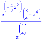
> sol:=c2*xi(2)+c4*xi(4);

We now verify that it does solve SE1:

> subs(f(x)=sol,SE1):

> simplify(%);

> evalb(%);

So we found an exact solution! Now we calculate the second-order energy correction using psi[1]:

> E2:=int(u0*sol*(W),x=-infinity..infinity);

> int(u0*sol*(W-E1),x=-infinity..infinity);

That is the exact answer! The two above calculations agree since u0 is orthogonal to sol, i.e., to psi[1].

Now do the same for the next equation: (H0-W0)*psi[2]=(E[1]-W)*psi[1]+E[2]*psi[0]

Note that it is only the right-hand side that changes!

> E1;

> RH2:=unapply(Int(expand(xi(m)*((E1-W)*sol+E2*u0)),x=-infinity..infinity),m):

> value(RH2(0));

> c2:=simplify(value(RH2(2))/2);

> c4:=simplify(value(RH2(4))/4);

> c6:=simplify(value(RH2(6))/6);

> c8:=simplify(value(RH2(8))/8);

> value(RH2(10));

All higher coefficients vanish. Note that we produced two more coefficients than before: this is due to the x^4 interaction, which can couple two adjacent columns or rows in the matrix that represents this interaction in the HO basis (generate the matrix representation and observe). There are four terms.

> sol2:=c2*xi(2)+c4*xi(4)+c6*xi(6)+c8*xi(8):

> SE2:=lhs(SE1)=((E1-W)*sol+E2*u0):

> subs(f(x)=sol2,SE2):

> simplify(%): evalb(%);

Let us check the orthogonality of the successive solution corrections:

> int(sol2*u0,x=-infinity..infinity);

> int(sol2*sol,x=-infinity..infinity);

Note that orthogonality to ground state is preserved. The solution psi[1] is not orthogonal to psi[2]. The orthogonality to the ground state means that the energy correction calculation can be made with W or with W displaced by some energy constant:

> E3:=int(u0*W*sol2,x=-infinity..infinity);

> int(u0*sol2*(W-E1),x=-infinity..infinity);

Now the fourth order:

> RH3:=unapply(Int(expand(xi(m)*((E1-W)*sol2+E2*sol+E3*u0)),x=-infinity..infinity),m):

> value(RH3(0));

> c2:=simplify(value(RH3(2))/2);

> c4:=simplify(value(RH3(4))/4);

> c6:=simplify(value(RH3(6))/6);

> c8:=simplify(value(RH3(8))/8);

> c10:=simplify(value(RH3(10))/10);

> c12:=simplify(value(RH3(12))/12);

> value(RH3(14));

All subsequent coefficients vanish. There are four terms in the solution:

> sol3:=c2*xi(2)+c4*xi(4)+c6*xi(6)+c8*xi(8)+c10*xi(10)+c12*xi(12):

> SE3:=lhs(SE1)=((E1-W)*sol2+E2*sol+E3*u0):

> subs(f(x)=sol3,SE3):

> simplify(%): evalb(%);

We continue to find exact solutions to the Dalgarno-Lewis equations, and we preserve the orthogonality to the ground state:

> int(sol3*u0,x=-infinity..infinity);

> int(sol2*sol3,x=-infinity..infinity);

Orthogonality to ground state is again preserved.

> E4:=int(u0*W*sol3,x=-infinity..infinity);

> int(u0*sol3*(W-E1),x=-infinity..infinity);

This is the fourth order. Now want the fifth! Our series expansion for the ground-state energy so far reads as:

> E0+lambda*E1+lambda^2*E2+lambda^3*E3+lambda^4*E4;

It is somewhat worrisome that the coefficients are growing...

> RH4:=unapply(Int(expand(xi(m)*((E1-W)*sol3+E2*sol2+E3*sol+E4*u0)),x=-infinity..infinity),m):

> value(RH4(0));

> c2:=simplify(value(RH4(2))/2);

> c4:=simplify(value(RH4(4))/4);

> c6:=simplify(value(RH4(6))/6);

> c8:=simplify(value(RH4(8))/8);

> c10:=simplify(value(RH4(10))/10);

> c12:=simplify(value(RH4(12))/12);

> c14:=simplify(value(RH4(14))/14);

> c16:=simplify(value(RH4(16))/16);

> c18:=simplify(value(RH4(18))/18);

> sol4:=c2*xi(2)+c4*xi(4)+c6*xi(6)+c8*xi(8)+c10*xi(10)+c12*xi(12)+c14*xi(14)+c16*xi(16):

> SE4:=lhs(SE1)=((E1-W)*sol3+E2*sol2+E3*sol+E4*u0):

> subs(f(x)=sol4,SE4):

> simplify(%): evalb(%);

> E5:=int(u0*W*sol4,x=-infinity..infinity);

> int(u0*sol4*(W-E1),x=-infinity..infinity);

Do one more, the sixth:

> RH5:=unapply(Int(expand(xi(m)*((E1-W)*sol4+E2*sol3+E3*sol2+E4*sol+E5*u0)),x=-infinity..infinity),m):

> value(RH5(0));

> c2:=simplify(value(RH5(2))/2);

> c4:=simplify(value(RH5(4))/4);

> c6:=simplify(value(RH5(6))/6);

> c8:=simplify(value(RH5(8))/8);

> c10:=simplify(value(RH5(10))/10);

> c12:=simplify(value(RH5(12))/12);

> c14:=simplify(value(RH5(14))/14);

> c16:=simplify(value(RH5(16))/16);

> c18:=simplify(value(RH5(18))/18);

> c20:=simplify(value(RH5(20))/20);

> c22:=simplify(value(RH5(22))/22);

> c24:=simplify(value(RH5(24))/24);

> sol5:=c2*xi(2)+c4*xi(4)+c6*xi(6)+c8*xi(8)+c10*xi(10)+c12*xi(12)+c14*xi(14)+c16*xi(16)+c18*xi(18)+c20*xi(20):

> SE5:=lhs(SE1)=((E1-W)*sol4+E2*sol3+E3*sol2+E4*sol+E5*u0):

> subs(f(x)=sol5,SE5):

> simplify(%): evalb(%);

> E6:=int(u0*W*sol5,x=-infinity..infinity);

And, one more:

> RH6:=unapply(Int(xi(m)*((E1-W)*sol5+E2*sol4+E3*sol3+E4*sol2+E5*sol+E6*u0),x=-infinity..infinity),m):

> value(RH6(0));

> c2:=simplify(value(RH6(2))/2);

> c4:=simplify(value(RH6(4))/4);

> c6:=simplify(value(RH6(6))/6);

> c8:=simplify(value(RH6(8))/8);

> c10:=simplify(value(RH6(10))/10);

> c12:=simplify(value(RH6(12))/12);

> c14:=simplify(value(RH6(14))/14);

> c16:=simplify(value(RH6(16))/16);

> c18:=simplify(value(RH6(18))/18);

> c20:=simplify(value(RH6(20))/20);

> c22:=simplify(value(RH6(22))/22);

> c24:=simplify(value(RH6(24))/24);

> c26:=simplify(value(RH6(26))/26);

> sol6:=c2*xi(2)+c4*xi(4)+c6*xi(6)+c8*xi(8)+c10*xi(10)+c12*xi(12)+c14*xi(14)+c16*xi(16)+c18*xi(18)+c20*xi(20)+c22*xi(22)+c24*xi(24):

> SE6:=lhs(SE1)=((E1-W)*sol5+E2*sol4+E3*sol3+E4*sol2+E5*sol+E6*u0):

> subs(f(x)=sol6,SE6):

> simplify(%): evalb(%);

> E7:=int(u0*sol6*(W-W1),x=-infinity..infinity);

This worrisome trend of growing coefficients has continued:

> E1,E2,E3,E4,E5,E6,E7;

> lambda:='lambda':

> EO2:=E0+E1*lambda+E2*lambda^2;

> EO3:=EO2+E3*lambda^3;

> EO4:=EO3+E4*lambda^4;

> EO5:=EO4+E5*lambda^5;

> EO6:=EO5+E6*lambda^6;

> EO7:=EO6+E7*lambda^7;

> plot([EO2,EO3,EO4,EO5,EO6,EO7],lambda=0..0.5,-2..2,color=[red,blue,green,black,grey,magenta]);

Let us find the exact eigenenergy at lambda=0.1 and compare the various approximations:

> E_num:=0.559145;

> SE:=-1/2*diff(u(x),x$2)+(1/2*x^2+1/10*x^4-E_num)*u(x)=0;

> solSE:=dsolve({SE,u(0)=1,D(u)(0)=0},u(x),numeric,output=listprocedure):

> ux:=subs(solSE,u(x)):

> plot('ux(x)',x=0..4,view=[0..4,-0.2..1]);

> Pt:=[[1,E0+0.1*E1],[2,subs(lambda=0.1,EO2)],[3,subs(lambda=0.1,EO3)],[4,subs(lambda=0.1,EO4)],[5,subs(lambda=0.1,EO5)],[6,subs(lambda=0.1,EO6)],[7,subs(lambda=0.1,EO7)]];

> plot([Pt,E_num],1..8);

Clearly this is an example where perturbation theory does not work! For the x^4 potential even a coupling of lambda=0.1 leads to a useless asymptotic series. For smaller lambda is should be useful, however.

> E_num:=0.514085;

> SE:=-1/2*diff(u(x),x$2)+(1/2*x^2+1/50*x^4-E_num)*u(x)=0;

> solSE:=dsolve({SE,u(0)=1,D(u)(0)=0},u(x),numeric,output=listprocedure):

> ux:=subs(solSE,u(x)):

> plot('ux(x)',x=0..4,view=[0..4,-0.2..1]);

> Pt:=[[1,E0+1/50*E1],[2,subs(lambda=1/50,EO2)],[3,subs(lambda=1/50,EO3)],[4,subs(lambda=1/50,EO4)],[5,subs(lambda=1/50,EO5)],[6,subs(lambda=1/50,EO6)],[7,subs(lambda=1/50,EO7)]];

> plot([Pt,E_num],1..8);

Eventually the expansion does diverge! The message is: for small coupling perturbation theory (even though it can result in a semi-convergent series) can be extremely useful. This is particularly true for problems where many terms of the expansion can be calculated symbolically or by numerical techniques.

Exercise 1:

Pick a different power-law potential (possibly a linear combination). Carry out the calculations and compare the results with exact solutions.

We can also look at the wavefunctions: one can see that they fail at moderate lambda, and then fail at large lambda [we show the one used to calculate the enegy correction E3, and the one for E5].

> u2:=u0+lambda*sol+lambda^2*sol2:

> u5:=u2+lambda^3*sol3+lambda^4*sol4+lambda^5*sol5:

> plot([subs(lambda=1/50,u2),subs(lambda=1/50,u5)],x=0..3,view=[0..3,-0.2..1],color=[red,blue]);

> plot([subs(lambda=1/10,u2),subs(lambda=1/10,u5)],x=0..3,view=[0..3,-0.2..1],color=[red,blue]);

We see that the higher wavefunction corrections are very small in the first case, and that they are destroying the state in the second example.

Can Pade approximants rescue the situation of the diverging series for the energy eigenvalue?

> with(numapprox):

> Pade:=pade(EO7,lambda,[3,4]);

> plot(Pade,lambda=0..1);

> subs(lambda=0.1,Pade);

This agrees rather well with the numerical result. Let us check a value at strong coupling:

> subs(lambda=1.,Pade);

> E_num:=0.80375;

> SE:=-1/2*diff(u(x),x$2)+(1/2*x^2+1*x^4-E_num)*u(x)=0;

> solSE:=dsolve({SE,u(0)=1,D(u)(0)=0},u(x),numeric,output=listprocedure):

> ux:=subs(solSE,u(x)):

> plot('ux(x)',x=0..4,view=[0..4,-0.2..1]);

We see that the Pade result based on the perturbation expansion to seventh order does not cure everything.

Exercise 2:

Carry out the perturbaton expansion to tenth order, construct a better Pade approximant and observe whether the ground-state eigenvalue can be obtained within 1% of the numerical value.

>