1. Select Student's t Demonstration from the main menu.
2. Enter the total Number of Samples you want the computer to randomly select (a number between 1,000 and 10,000).
3. Enter the Sample Size -- the number of observations that you want the computer to select for each sample (a number between 2 and 40).
4. Choose the population from which the computer draws its samples (normal, uniform, triangular or v-shaped).
5. Choose OK and the computer will build the distribution of t scores. Before the computer adds a point to the distribution, it shows you the values that yield each t score, and the value of the t score itself (so long as you have selected a sample size between 2 and 10). Pressing the number keys 1 - 9 will cause a delay of from 1 /10 to 8 seconds , respectively, for each sample. If you press the 0 (zero) key, the demonstration will finish as fast as possible. Pressing the Escape key will abort the demonstration. When the End key is pressed, the computer displays a dialog box, "Pause Again?", and pauses until any key is pressed or 'YES' or 'NO' is clicked -- If 'YES' was clicked or the End key was pressed again, the computer pauses again.
Your selections will be displayed in the top corners of the window, and the Student's t Distribution will begin to form. If you have selected a sample size between 2 and 10, then, for each sample, the computer displays the values that it has randomly selected as well as their mean and t-score. For sample sizes greater than 10 only the t-score is displayed. Each t-score calculated will be plotted in the new distribution. When the computer is building the distribution, pressing the number keys 1 - 9 will cause a delay of 1 to 9 half-seconds , respectively, for each sample. If you press the 0 (zero) key, the demonstration will finish as fast as possible
When the t distribution is complete, the computer superimposes two curves onto the t distribution. The red curve is the theoretical curve of the normal distribution, and the white curve is the theoretical curve of the t distribution.
The purpose of Student's t Demonstration is to demonstrate various aspects of the distribution of the test statistic, Student's t. These are:
1. That the distribution of Student's t will approach a normal distribution when samples are drawn from a normal population;
2. That there is a family of Student's t score distributions.
We will use the same example that we used in the Central Limit Demonstration to elaborate on the distribution of Student's t. Imagine again that you are a student in Dr. D. Mented's Introductory Statistics class. As you know, this is a popular course because Prof. D. Mented starts the course by giving everyone a passing grade (50/100). But Dr. D. Mented's generosity ends there. The course is full of pop quizzes, which always have 10 questions, each worth half a mark. Depending on the quality of the answer, each question can earn a maximum of half a mark. But, if the answer is really terrible, students can also lose up to a half mark. So, scores on the pop quizzes can range from -5 to 5 marks. If a student completely flunks a pop quiz, 5 marks are taken away from their starting mark of 50!
D. Mented has been teaching stats for 45 years using this method, and has saved the marks from all of her students pop quizzes. We know nothing about how this population of quiz scores is distributed, other than that it has a mean (mu) of 0. If we wanted to use this population of scores to demonstrate the distribution of Student's t, this is what we'd do:
a. We'd first decide what sample size we were going to use to make a new distribution: a distribution of Student's t. Let's use n=9 (df = 8).
b. Next we'd randomly select 9 quiz scores, and calculate the mean. Then we'd calculate t: the distances of that sample mean from the population mean (mu) of 0, in standard deviation units. Then we'd draw another 9 scores, calculate the mean of that sample, calculate t for that sample mean, and so on, until we had randomly sampled as many samples as pratical (the computer limits you to 10,000 samples).
c. The t scores that we calculated in Step b are plotted in a new distribution: the distribution of Student's t. This is the kind of distribution that you build when you run the Student's t Demonstration after selecting the size of the random samples, the number of samples to draw, and the shape of the population distribution from which to draw the samples.
The Normality Assumption and Sample Size
T-tests assume that the population from which samples are drawn is normally distributed. If you draw a sample from a population that is not normally distributed, you may be in the position of biasing either in favour of, or against, finding a significant result. Try sampling with a small sample size (n=2) from each of the four populations . You will see that the t distribution generated by samples drawn from a normal population best approximates a normal shape. The t test is also said to be "robust" against violations of this assumption, so long as the sample size is large (n>=30). Try the same demonstration with larger sample sizes. With respect to the non-normal and symmetrical distributions (v-shaped and uniform), with larger sample sizes, the departure from an idealized t and normal curve is less marked. However, sampling from the non-symmetrical distribution (triangular) still biases in favour of a larger t value.
Student's t as a Family of Distributions
Student's t is said to be distributed as a family of distributions because the shape of the distribution changes with sample size. Try sampling from the normal population with varying sample sizes (e.g., 2, 10, 20, 30, etc.). You will see that varying sample size changes the shape of the t distribution, such that with increasing sample size (df), the departure from normality decreases. With sample sizes greater than 122, there is no difference between the t distribution and the distribution of z scores. This is why, when df is greater than 120, the critical value of the t statistic is identical to the critical value of z, i.e., the area under the curve for given values of t and z is identical. You can see this in the distributions that you generate with varying sample sizes. Look at the tails of the distribution -- the smaller the sample size, the greater the area is under the tails. Therefore, more extreme t-values will be required for significance with smaller sample sizes (df).
We calculate t in order to express our sample mean as a measure of how far that sample mean is from mu in standard deviation units. Remember that when we calculate Student's t, we don't know anything about the population from which the sample is drawn, other than the value of its mean (mu). In order to know how far our sample mean is from the population mean, we first have to know how as many samples as pratical from the population would be distributed. When we know how all means would be distributed, then we can easily say that our mean is so many standard deviations from the population mean. When we know the population standard deviation, we know that the Distribution of Sample Means is normally distributed and has a mean equal to that of the population, and that it has a standard error equal to the population standard deviation divided by the square root of our sample size. (If this point is not clear consult the Teacher's PET on the Central Limit Demonstration.) To convert any particular sample mean into a standard score that expresses how far that sample mean is from the population mean (mu) in standard deviation units (z), we simply divide the distance between the two means by the standard error of the Distribution of Sample means. We know that this distribution would have a mean of 0 and a standard error equal to the population standard deviation divided by the square root of the sample size. (If this point is unclear, consult the teacher's PET on the Distribution of z.)
In the case of t, we don't know the population standard deviation, and hence, we don't know what the standard error of the t distribution will be when we randomly sample as many samples as pratical of a particular size. In this case, we have to estimate the population standard deviation (and hence the standard error of the t distribution). The population standard deviation is estimated from the sample standard deviation and therefore will vary from sample to sample.
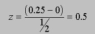
If you were going to compute z scores for as many samples as pratical of a particular size from a population with a known standard deviation, then the denominator of the z ratio would be a constant. Every sample that you drew that had the same mean would also have the same z score associated with it. For example, you could draw from Dr. D. Mented's population of quiz scores the following samples: -2, -4, 3, 4, (mean = 0.25) and -3, 0, 4, 0 (mean = 0.25). Assuming that the mean of Dr. D. Mented's population is 0 and the standard deviation is 1, we can calculate a z score of 0.5 for both of these examples: for the first sample
and for the second sample
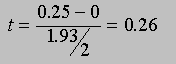
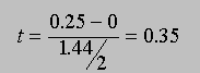
Now let's assume that we don't know the standard deviation of Prof. D. Mented's population (but we do know that the mean is 0). Now we have to calculate t using the sample standard deviations as an estimate of the population standard deviation. For the first sample, s = 1.93, and for the second sample, s = 1.44. For the first sample, we would calculate
and for the second sample, we would calculate
The t distribution has more variability than the z distribution -- for smaller sample sizes it is flatter than a normal distribution and more spread out. With sample sizes greater than 122, there is no difference between the t distribution and the distribution of z scores. This is why, when df is greater than 120, the critical value of the t statistic is identical to the critical value of z, i.e., the area under the curve for given values of t and z is identical. You can see this in the distributions that you generate with varying sample sizes. Look at the tails of the distribution -- the smaller the sample size, the greater the area is under the tails. Therefore, more extreme t-values will be required for significance with smaller sample sizes (df). So, the t distribution is really a family of distributions, one distribution for each sample size from n=2 (df =1) to 121(df =120), and one t distribution for sample sizes >=122 (df >120).