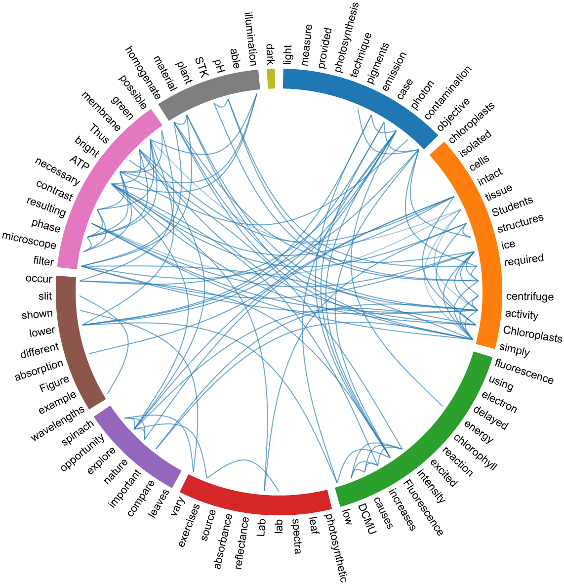
| Figure 2. Light Outcomes |
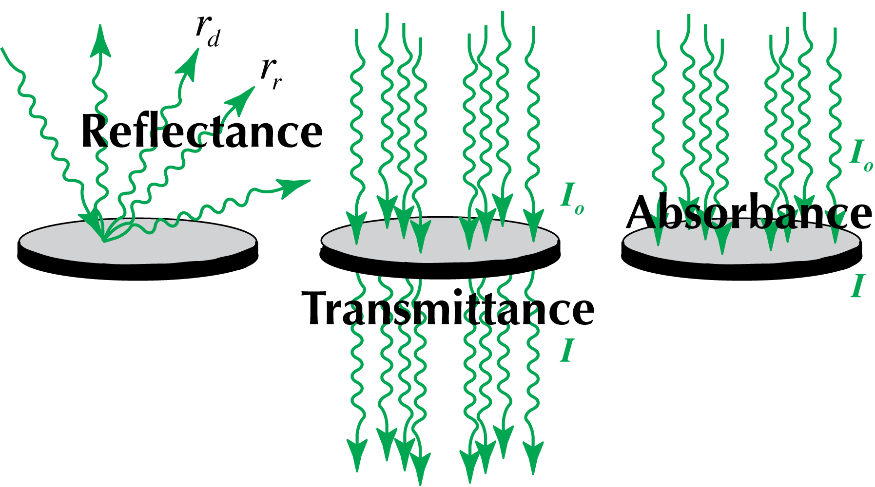 |
There are three ways that light can interact with a photosynthetic organ (such as a leaf) (Figure 2). The first of these is reflection, simply rebounding off of the leaf surface and therefore never utilized in leaf photosynthesis. Reflectance (R) comes in various forms. The simplest is regular reflection (rr), where the incident light is reflected off of the leaf at the same angle (that is, the incident angle is equal to the angle of reflection). This will occur with very smooth surfaces, but is less likely to happen if the leaf surface is rough (as it usually is, at least at a microscopic level). In the latter case, the reflectance is diffuse (rd). Thus, to a first approximation: R = rr + rd (total reflectance is the sum of regular and diffuse reflectance).
| Figure 3. Pathways of Internal Reflectance |
 |
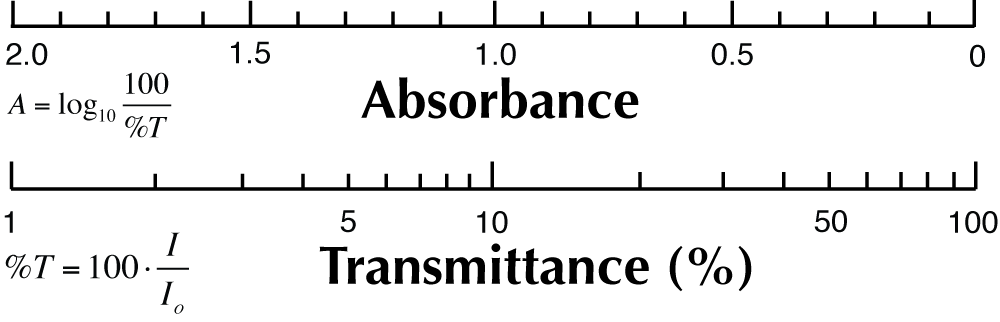
| Figure 4. Absorbance and Transmittance Scales |
 |
Absorbed + Reflected + Transmitted = 1
The equation as written indicates that all the light impinging on the leaf is conserved. Missing is yet another complication! Fluorescence does occur, which is the release of photon energy (in the form of longer wavelength light) after light absorption. This is so important in photosynthesis research that we will explore it in a separate lab exercise.
In your lab exercises, you will have the opportunity to measure reflectance, transmittance and absorbance, and fluorescence: All four as a function of the wavelength of light. Is this important? Very much so. For one thing, it reveals the relation between the photosynthetic organ and how it interacts with light, the basic events leading to photosynthesis. For another, it provides the fundamental knowledge necessary for remote sensing of biotic health, by satellites for example. This is how crop productivity is documented annually. A basic understanding of the fates of light has diverse and economically important relevance.
Lab 01 Spectral Properties of Intact Leaves
Reflectance Spectroscopy
| Figure 1. Reflectance Spectra. You may wish to refer to this figure during the lab to relate wavelength and color. |
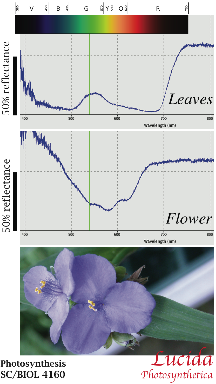 |
Examples of reflectance spectra are shown in Figure 1: Both a leaf (upper panel) and a flower (lower panel). Your spectra should look similar. Note that the reflectance is shown as a percent for calibrated measurements.
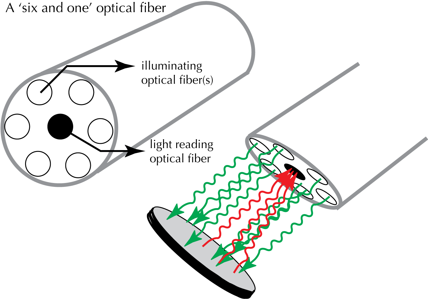
For measurements of reflectance spectra, you will be using a probe that operates as shown in Figure 2. Light is provided from a tungsten-halogen light source (an incandescent light source which provides broad spectral 'white light') through a ring of 6 optical fibers. The reflected light passes through a light reading optical fiber to a diffraction grating that separates the 'colors' (wavelengths) of the reflected light, thereby creating the wavelength spectrum of reflected light
| Figure 2. Reflectance Measurement |
 |
It is crucial to calibrate the reflectance probe prior to use! This is done using a 'white' reflector called a reflectance standard (that reflects all wavelengths of light) to adjust 'maximum output', and 'no light' to adjust the 'dark' baseline. Please be sure to perform the calibrations during the initial setup, following the procedures indicated in the calibration section [http://biologywiki.apps01.yorku.ca/index.php?title=Main_Page/BIOL_4160/Spectral_Properties_of_Intact_Leaves#Reflectance_Spectra_Measurements_--Calibration].
The leaves that you choose to measure are your decision. Make sure you indicate the species, and any special characteristics. For example, is it a grass leaf? A succulent? Is it colored with pigments other than chlorophyll? Some leaves may be 'hairy', and you should take note of this as well, as it may affect the spectral properties of the leaf.
Make measurements of reflectance from both the upper surface and the lower surface of the leaves you select. Are they different? Why?
You may notice strong reflection in the infrared region of the spectra. Feel free to compare it with your own reflectance spectrum (from your skin)! This may provide insight into the very different radiant energy balances of a human and a leaf. You can even test your clothing if you want: to get a better sense of the diversity of reflectance spectra.
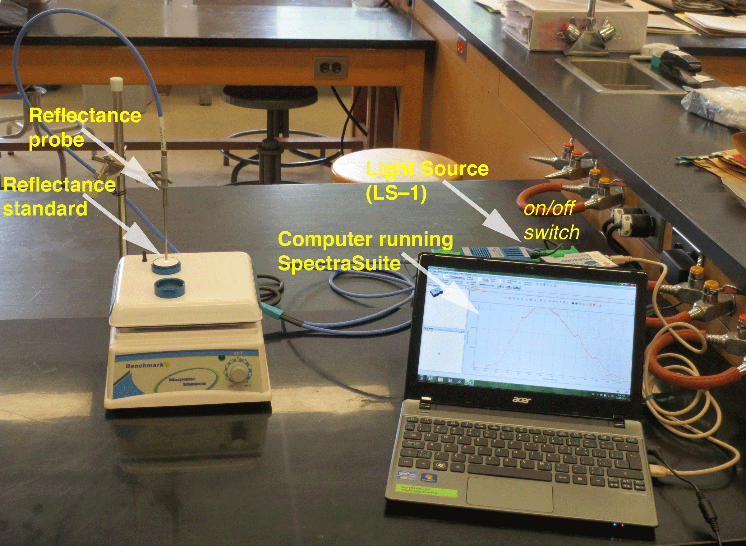
| Figure 3. Reflectance Workstation |
 |
Be sure to save the spectra you obtain, and keep careful notes of what you did.
Absorbance and Transmittance Spectroscopy
Once you have obtained reflectance spectra, you will need to measure the absorbance and transmittance spectra. For these, you need to provide a light source on one side of the leaf while you measure the absorbance through the leaf. It is vitally important that you ensure the distance from the light source to the probe is kept constant, while you compare the spectra with the leaf intercepting the light, versus no interception. Again, you must calibrate the probe before performing your measurements: adjusting the maximum output for the lamp source, and the dark baseline. Also, you need to measure the thickness of the leaf. Absorption depends upon the depth of the material. Doubling the thickness causes a doubling of the absorbance. This is very important when you are comparing two different kinds of leaves.
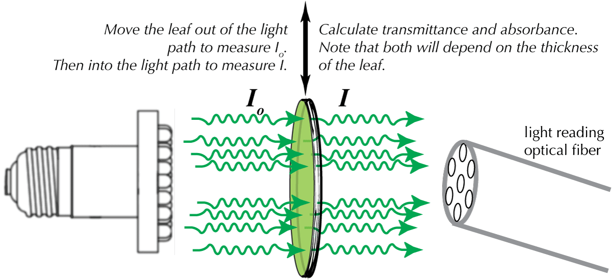
| Figure 4. Transmittance Measurement |
 |
A number of different light sources will be provided for you. Some are specific colors (LED lamps), or 'white' (incandescent) light sources. Choose the white source and two others for your transmittance measurements for the leaves you selected for reflectance measurements. Please be careful that you do not 'contaminate' your spectra with ambient lighting. Fluorescent lamps emit light at very specific wavelengths. You can minimize contamination using cardboard or light-proof cloth.
For leaf absorbance measurements, your light source intensity should not be too high, since it will be difficult to measure absorbance in the very thin leaf, because the ratio of I to Io will be near 1 if the lamp is very bright. If you can't distinguish the spectra with and without the leaf, put more leaves in the light path. Do measurements of both absorbance and transmittance (calibrating the probe each time). Figure 4 provides a general schematic of the technique. Recall from the introductory section [http://biologywiki.apps01.yorku.ca/index.php?title=Main_Page/BIOL_4160/Origins_and_Fate_of_Light] that transmittance and absorbance are related: both compare the ratio of I and Io. Transmittance as a percent: (100(I/Io). Absorbance as a log: (log(Io/I).
Hypotheses and Observations:
The observations you make should be similar for all lab groups. What will vary is your decision about the photosynthetic leaf you use, and the light sources for absorbance and transmittance. You have the opportunity to propose your own hypotheses. For example, is infrared reflectance important? Does it differ between a succulent leaf, adapted to desert conditions, and a shade leaf adapted to low light conditions? What about the position of the leaf in the plant, shaded versus un-shaded? What would you hypothesize? Does leaf pigmentation (besides chlorophyll) have an impact?
Finally, in the introduction [http://biologywiki.apps01.yorku.ca/index.php?title=Main_Page/BIOL_4160/Origins_and_Fate_of_Light], you were provided with an ideal summary of the fates of light:
Absorbed + Reflected + Transmitted = 1
Quantifying this is not so simple (this is why calibrations are so important), but your data should provide you with sufficient information to estimate the relative contributions of each. Quantifying on the basis of percentages is the best approach. Be sure to correct for the thickness of the leaves, if required. If you focus on PAR (photosynthetically active radiation: 400-700 nm), what you are measuring is how effective leaves are at absorbing light energy for photosynthesis.
Reflectance Spectra Measurements --Setup
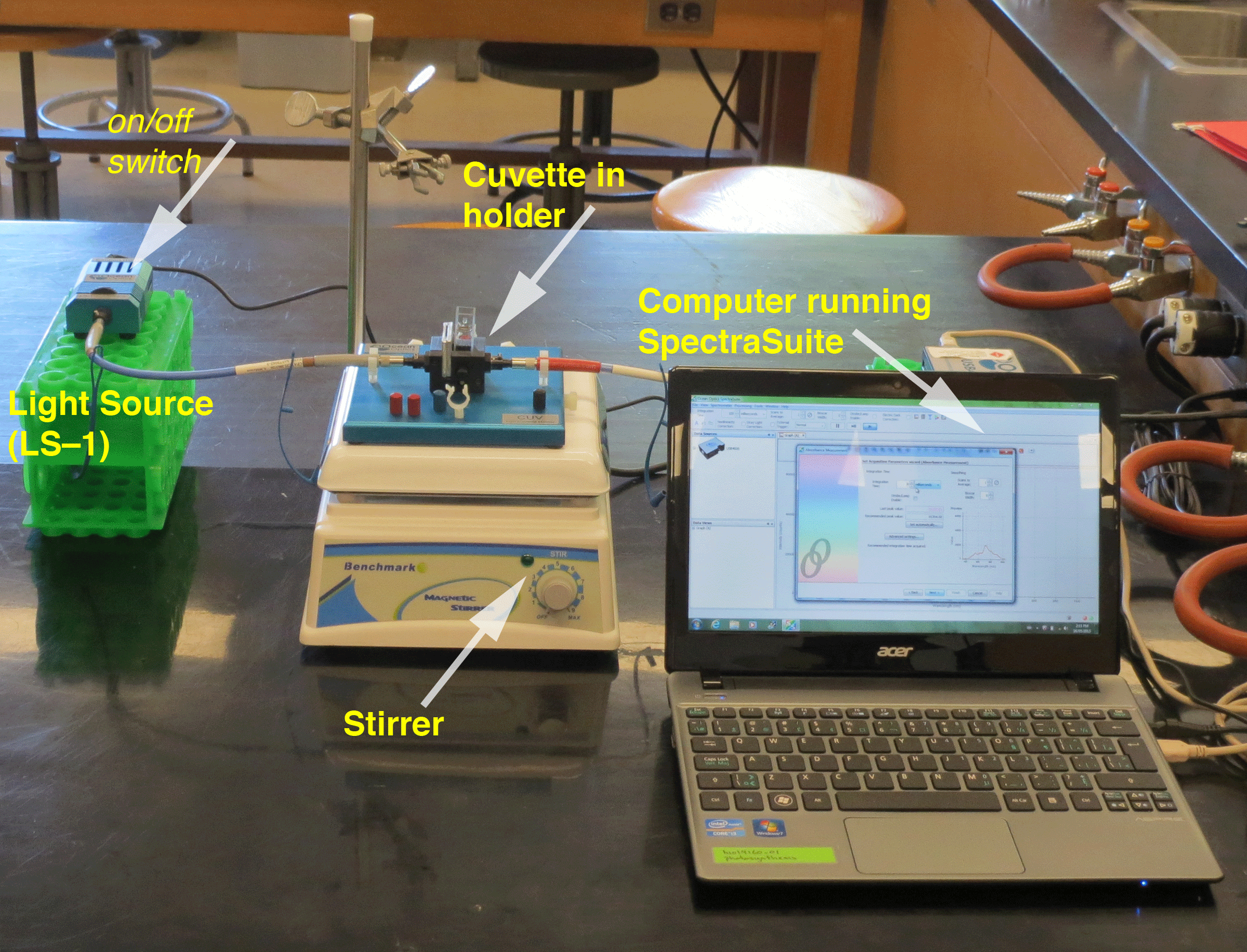
The instrumentation should be setup for you, but here is a detailed description for reference purposes. The instrumentation setup includes the computer running the SpectraSuite software. The computer is connected to the spectrometer via a USB cable. One of the fiber optic leads is connected to the spectrometer. The other is connected to the light source (a tungsten halogen lamp). The light source can be hot, so be careful touching the housing. The fiber optic cables can be damaged by over-bending, so be gentle. The two fiber optic leads merge into the cable connected to the reflectance probe. Note that the probe is measuring the spectra form a reflectance standard --part of the calibration procedure.
| Figure 5. Reflectance Setup (showing all the components) |
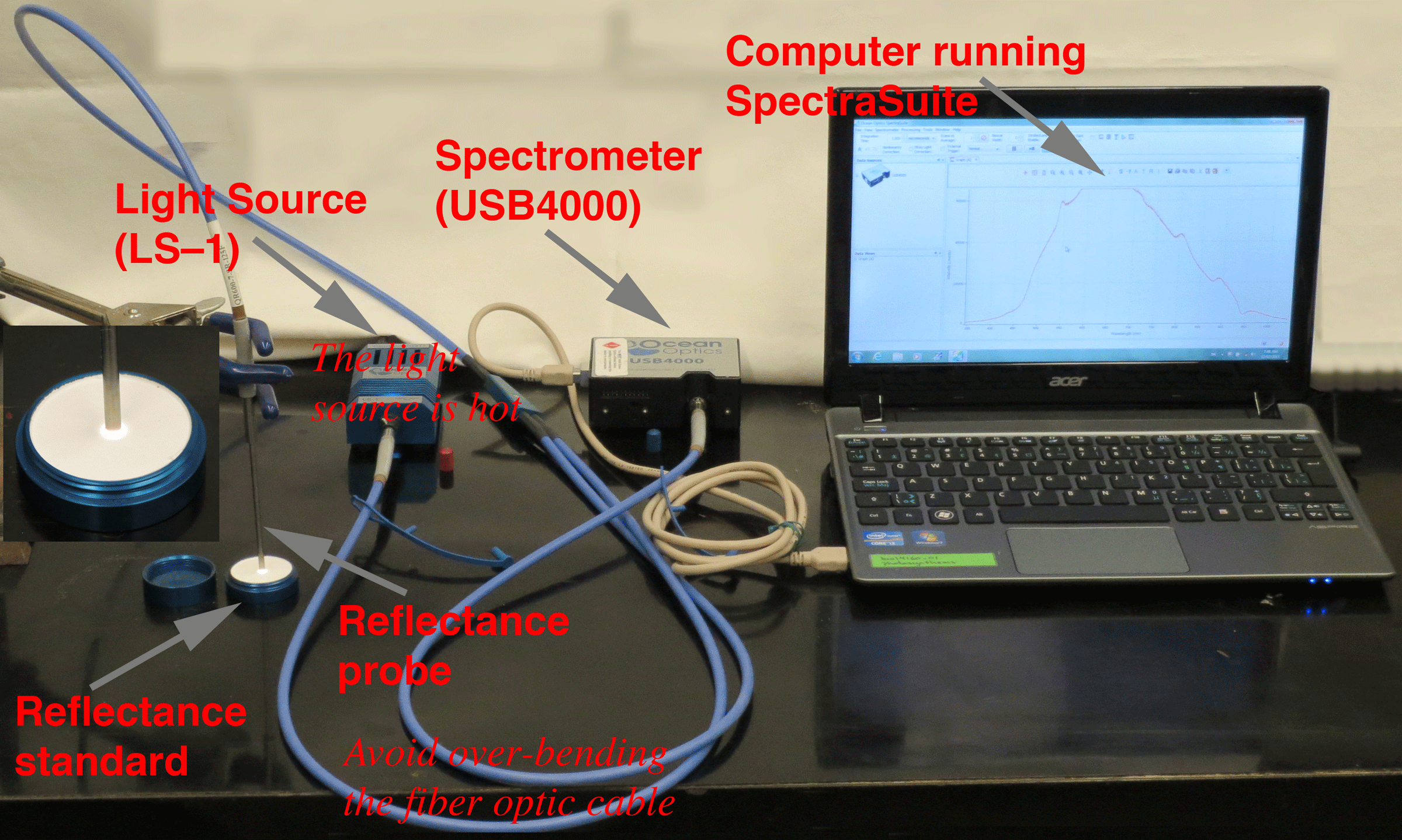 |
There are some crucial points to bear in mind when you setup the apparatus.
- Make sure you shield the reflectance standard and leaf from extraneous illumination. This can be reflected into the probe causing a spurious increase in reflectance. You should be able to determine whether this is a problem by monitoring the probe output with or without shading.
- Make sure that the distance between the probe and the leaf (and the reflectance standard) is constant. You can test for the effect of distance yourself to see how much of a difference it makes. The optics underneath the distance effect is complex, related to the angular spread of light --from the source and being sampled by the probe. So as close as possible is optimal, gently touching the material, but be careful not to damage the tip of the probe.
- Be sure to place the leaf on a black, non-absorbing surface to minimize reflection (and therefore contamination of the reflected light with transmitted light).
Reflectance Spectra Measurements --Calibration
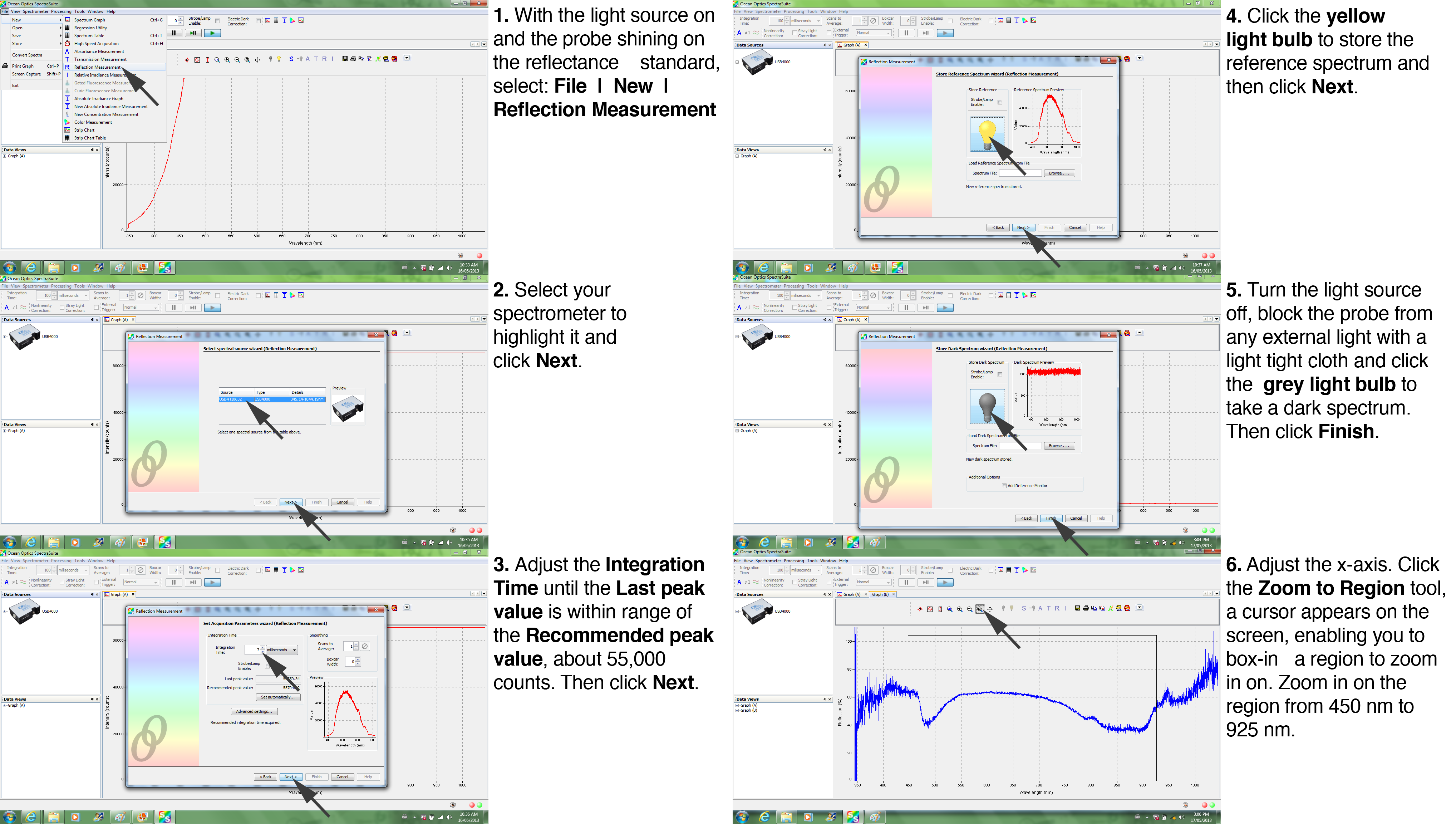
The calibration is important for quantitative comparisons. Note that it is necessary to turn the classroom lights off during the calibration steps. The calibration steps are shown below in Figure 7. First, turn the light source on (the switch is on the back of the LS-1 unit). Select File | New | Reflection Measurement. Highlight the spectrometer and click Next. Then, adjust the Integration Time until the Last peak value is within range of the Recommended peak value, about 55,000 (this doesn't have to be exact, just in the range: 45,000 is fine, 60,000 is too much). This ensures that the signal does not 'clip' at a level higher than the maximum measurable by the spectrometer. In the next steps, you record the spectra with the light bulb still 'on', then with the light bulb 'off.' For the latter, you need to turn off the light source (the switch is on the back of the LS-1 unit) and shade the probe from stray light with a light tight cloth. First, with the light still on click the yellow light bulb to store the reference spectrum and click Next. Turn off the light source to take a dark spectrum. The graph appears on the right side of the screen. Click the grey light bulb then Finish. Lastly, adjust the scaling on the x-axis (wavelength) by zooming in on the region of interest, 450 nm to 925 nm. You are now ready to bring your leaves to the table for your measurements of the reflectance spectra.
| Figure 7. Reflectance Calibration Tutorial |
 |
Absorbance and Transmittance Spectra Measurements --Setup and Calibration
The procedures for absorbance and transmittance measurements are similar to the reflectance measurements. However, the probe should by pointing to the side (horizontally) rather than down. And, the LS-1 light source must be turned off. For an incandescent light source (white light), the steps in the calibration procedure are also similar --but now you start by selecting File | New | Transmission Measurement or File | New | Absorbance Measurement and proceed from there. For the LED lamps (blue, red, green and 'white'), calibration is difficult because of the narrow band of the LED light. So, simply measuring the light intensity with (I) or without (Io) the leaf in the light path may be the best option. The intensities (I and Io)can be used to calculate transmittance and/or absorbance.
Hints and Suggestions for the Discerning Experimentalist
It can be difficult to control the light intensity so that it falls into the correct range. In addition to adjusting the integration time, you can shift the lamp to adjust output (but be sure you don't move the lamp once you begin your measurements!).
If the output is 'noisy', you can decrease the noise by averaging the scans. This will to increase the time required to obtain the spectra, so avoid too much averaging (averaging 8 scans should be sufficient to 'de-noise' the scans if noise is a problem). The box for adjusting the Scans to Average is near the upper left corner of the SpectraSuite window.
For the LED lamps, the spectral output is very narrow. This can cause problems if you try and calibrate the lamps, because the very small signals at wavelengths shorter than or longer than the spectral output of the lamp causes a very low signal to noise ratio and therefore a lot of noise. It's easier to just use the intensity output of the spectrometer without doing a calibration: either graph A in the software or restarting the SpectraSuite software will bring you back to the intensity output default. The transmission and absorbance has to be calculated manually (per the Origins and Fate of Light Introduction at [http://biologywiki.apps01.yorku.ca/index.php?title=Main_Page/BIOL_4160/Origins_and_Fate_of_Light]), but this is easy to do.
Data Files
To upload data files...
- log into the lab student account (the TA will provide you with the account information)
- click on 'Upload file' under the toolbox section (left side of the webpage)
- you will be re-directed to http://biologywiki.apps01.yorku.ca/index.php?title=Special:Upload
- upload your data file (be sure to provide information about the file to help other students using your data)
- the uploaded data files will be listed at http://biologywiki.apps01.yorku.ca/index.php?title=Special:ListFiles
Student Results (September 2013)
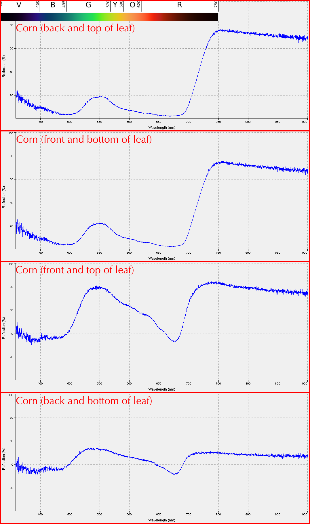
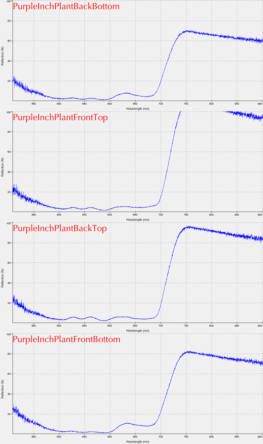
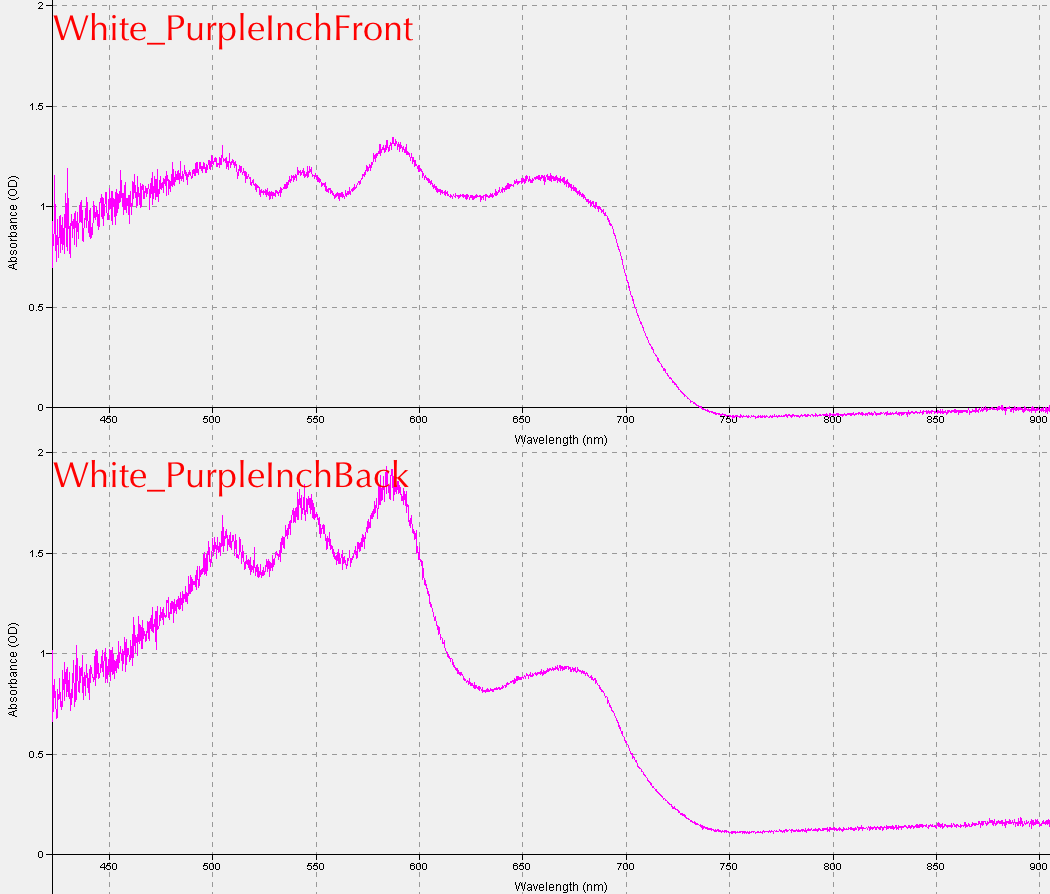
These are some examples of the results students obtained from the first lab exercise: Reflectance for corn (left) and a "Purple Inch Plant" (right).
Absorbance for the "Purple Plant" is shown below.
Lab 02 Visualizing the Photosynthetic Apparatus
Introduction
So far, you have had an opportunity to explore the nature of light and its fates in intact photosynthetic organs (leaves). In eukaryotic cells, photosynthesis occurs in chloroplasts. Chloroplasts are a unique organelle, containing their own DNA and the full suite of biochemical reactions required to convert light energy to carbohydrate.
In this lab, you will have the opportunity to visualize the photosynthetic apparatus and become familiar with the nature of the chloroplast organelle in a variety of photosynthetic organisms. Part of the lab objective is to compare the structure of chloroplasts in situ with their structure in vitro. Most biochemical experiments on chloroplasts require that the chloroplasts be isolated (in vitro). Thus, you will be required to isolate chloroplasts from a photosynthetic tissue (spinach leaves and algal cells) and compare these in vitro chloroplasts to in vivo chloroplasts in leaves and algal organisms cultured in the Biology Department for teaching and research.
To visualize the chloroplasts, you will take advantage of a fourth fate for a light photon interacting with the photosynthetic apparatus: fluorescence.
Microscopy
With the microscope, it will be possible to identify and measure the size of chloroplasts. You will be using bright field, phase contrast, and fluorescent microscopy and should diagram (with scales) and comment on the structures you observe with the three microscopic techniques.
It will be necessary to calibrate the microscope using a micrometer slide. Kohler illumination is crucial for optimal viewing using bright field and phase contrast. You will have had experience doing this in previous biology labs, but can request assistance from the lab demonstrator as required.
Chloroplast Isolation
Practically all biochemical assays of photosynthesis use isolated chloroplasts, in part to avoid 'contamination' with other cell organelles, especially mitochondria. Historically, careful isolation of 'pure' chloroplasts was necessary for biochemists to accurately characterize what chloroplasts do. To isolate the chloroplasts, it is necessary to break apart the tissue to the extent that individual chloroplasts are released from the cell. A typical technique to disrupt cells is a blender. It is highly effective, but has to be used with care since excessive homogenization will damage the chloroplasts (something you could assess using microscopy). An alternative is a mortar and pestle, a gentler technique that minimizes damage --we will use a mortar and pestle in this (and future) experiments. The chloroplast in situ exists in an osmotically and pH balanced environment. Thus, the tissue should be disrupted in a solution that mimics the osmolarity (about 600 mosmol/kg, sucrose is often used) and pH (about 7.2, tricine is a common buffer) of the cytoplasm. A common media used for chloroplast isolation is STK (sucrose/tricine/KCl).
STK (pre-chilled on ice):
- Sucrose (FW 342.3) 0.6 M
- Tricine (FW 179.2) 0.05 M
- KCl (FW 74.55) 0.02 M)
Other materials: Spinach, Mortar and pestle (pre-chilled on ice), Algal cultures, Glass homogenizer (pre-chilled on ice), Cheesecloth (to filter the homogenates), Centrifuge and centrifuge tubes (to pellet the chloroplasts), and Miscellany (beakers, No. 1 filter paper etc.)
Pre-chilling is important because, once isolated from the tissue, the chloroplasts will be subjected to proteolytic and lipolytic activity, resulting in a progressive deterioration of the organelles. Chilling inhibits the deterioration.
Chloroplast Preparation from Spinach
Please note that this is the longest procedure you will have to undertake in this laboratory. It is also the most important, in the sense that you will be isolating chloroplasts from spinach in a number of labs. This is a case of engaging in real scientific practice: learning a procedure and repeating it until (in the words of previous students in this course) you can "isolate chloroplasts with your eyes closed" (but please don't try! Keeping your eyes open is very helpful!).
When you harvest the spinach leaves, try to minimize wilting, because wilting has an adverse effect on the yield of healthy chloroplasts. Wash the spinach leaves thoroughly under tap water, and remove midribs etc. with scissors (or a razor). Be sure to set aside leaves (still on the spinach plant) for subsequent viewing under the microscope. Cut the leaves into squares of about 2 cm. Place about 10 grams in the mortar, and cover with 50-100 ml of STK. Homogenize by crushing the leaves with the pestle using a circular motion until homogenized (about 1-3 minutes). Take the homogenate and filter through three layers of cheesecloth into a beaker pre-chilled on ice. The filtrate should be centrifuged at about 500 X g for 2-3 minutes to remove debris. The supernatant should be centrifuged at about 10,000 X g for 10 minutes to pellet the chloroplasts. Decant the supernatant and re-suspend the chloroplasts in a small volume of STK.
It is always crucial to assure that the centrifuge tubes are balanced. That is, the same weight in each of the two tubes that are placed in holders on opposite sides of the centrifuge rotor.
Below is a step-by-step flow chart for the isolation of chloroplasts from spinach:
Constructing a Flow ChartWhile researchers rely upon written protocols similar to the one presented above, when working at the bench, they will usually prepare a flow chart similar to the one at right. You will find such flow charts helpful over the course of the term, especially as lab exercises become more complex. |
|
Chloroplast Preparation from Algae
When you harvest the algal cultures, the technique for isolating chloroplasts will vary depending on the type of algae. If you are provided with Chara australis, it is as simple as cutting one end of the internode cell (with small scissors) and squeezing the cell sap (with chloroplasts) onto a microscope slide.
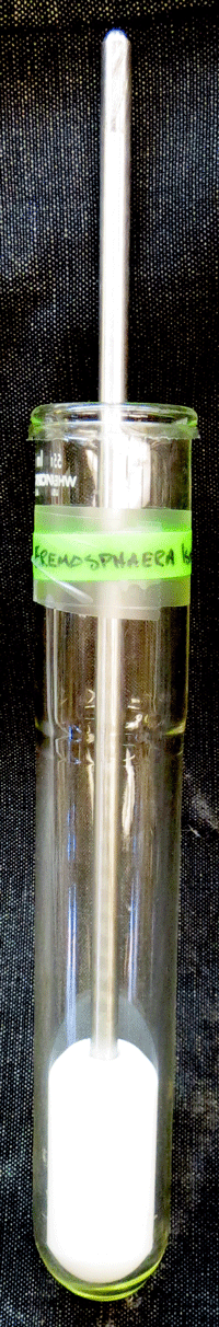

If you are provided with Eremosphaera viridis, the large cells need to be broken apart. This is done with a glass mortar and pestle. The cells are decanted from the culture flask into a 50 ml disposable centrifuge tube, allowed to settle (this will take less than 5 minutes at "1 X g"). The supernatent (culture media) is carefully poured off (into the sink) and the cells re-suspended in STK. Then, they are poured into the glass homogenizer (Figure 1). The plunger is pushed to the bottom while twisting it. This is repeated 4 times, at which point the cells will have been disrupted, releasing the chloroplasts. The homogenate is filtered through multiple layers of cheesecloth, and the filtrate (chloroplast rich) is used as is for microscope visualization.
For all of the plant material, first observed the intact leaf or cell under the microscope, using bright-field, phase contrast, and fluorescence. Take careful note of the structure of the chloroplasts in situ. In the case of leaves, it is often useful to peel the epidermis off the leaf, and view the leaf with the peeled side up. On the microscope slide, samples of leaves can covered with pure water, and algal material can be covered with a drop of the culture medium. Chloroplasts should be covered with STK. Compare the intact leaves or cells with the isolated chloroplasts.
Under bright field illumination, you should be able to measure the size of chloroplasts in the various tissues (chloroplast will be identifiable by their 'green' color).
With phase contrast, you may be able to discern a phase halo around chloroplasts in situ. Compare this with the presence (or absence) of a strong halo around isolated chloroplasts. The phase halo is caused by the close apposition of two membranes in intact chloroplasts. Thylakoids will not have a strong halo since they have only one membrane. This is one way to assess the 'intactness' of the isolated chloroplasts. Fluorescence allows you to obtain direct evidence for the presence of chlorophyll, the only strongly fluorescent pigment in photosynthetic tissue.
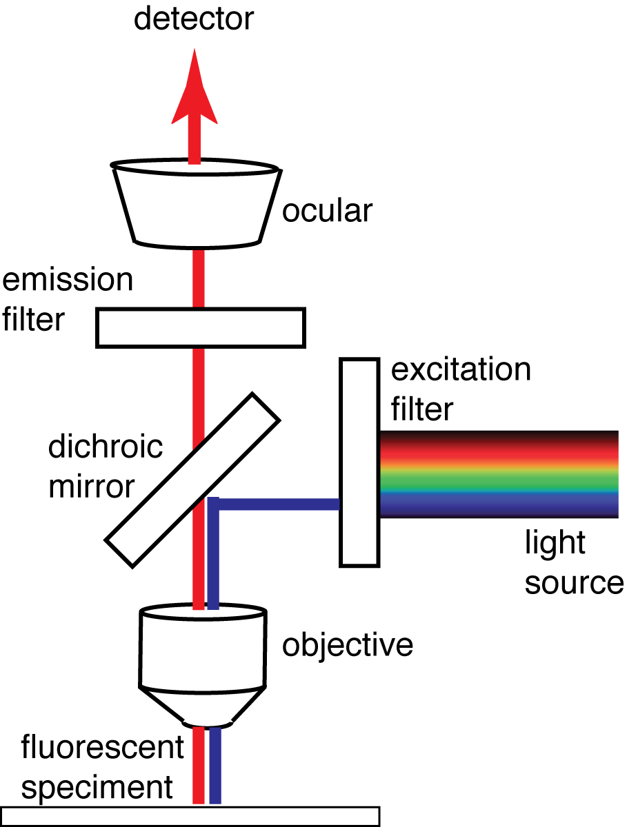
How Fluorescence Microscopy WorksThe technique used in microscopy is known as epi-fluorescence. Light of a wavelength suitable to excite a pigment (chlorophyll in our case) is transmitted through the objective with a dichroic filter --which reflects specific wavelengths, and allows others to pass through. The fluorescence light emitted from the pigment is focussed through the objective and selectively viewed with the emission filter (transmitting red light in the case of chlorophyll). Diagram re-drawn from Wikipedia: en.wikipedia.org/wiki/Fluorescence_microscope |
 |
With epi-fluorescence microscopy, you should be able to observe chlorophyll fluorescence in situ and in vitro. On the basis of your observations, compare the intactness of isolated chloroplasts with chloroplasts in situ.
For isolated chloroplasts, you simply take a drop of the suspension, place on a glass microscope slide and gently place a cover slip on top.
For in situ chloroplasts (in the leaf), the challenge is to slice through the leaf so that you will be able to see structures at the bottom and top of the leaf. One technique is to slice at a diagonal through the leaf. Another technique is to 'peel' the epidermis so that you can look directly at the internal architecture. Carefully place the leaf slices on a glass microscope slide, add a drop of water, and gently place a cover slip on top.
Hypotheses and Observations
The observations you make are qualitative in nature. For intact tissues and cells, how does the positioning and density of the chloroplasts relate to what you know about the spectral properties of intact leaves? Are chloroplasts dense enough? Would you predict 100% absorbance based upon their distribution in the leaf? For isolated chloroplasts, how do they compare with chloroplasts in situ? Would you predict that damage will affect the nature of the biochemical reactions the chloroplasts are capable of performing? For this question, take note that the light reactions are located on thylakoid membranes, carbon dioxide fixation and the Calvin cycle are located in the stroma of intact chloroplasts.
Data Files
To upload data files...
- log into the lab student account (the TA will provide you with the account information)
- click on 'Upload file' under the toolbox section (left side of the webpage)
- you will be re-directed to http://biologywiki.apps01.yorku.ca/index.php?title=Special:Upload
- upload your data file (be sure to provide information about the file to help other students using your data)
- the uploaded data files will be listed at http://biologywiki.apps01.yorku.ca/index.php?title=Special:ListFiles
Visualizing Chloroplasts in situ
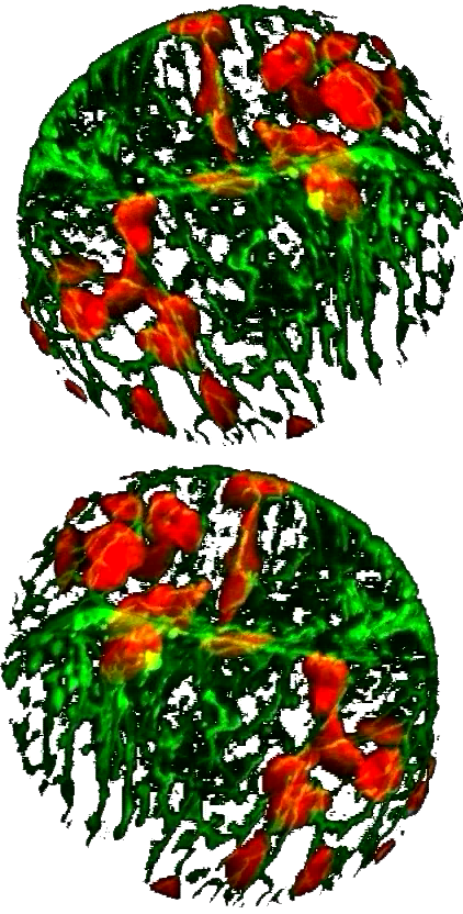
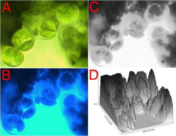 One aspect of visualizing the photosynthesis apparatus is the question 'how efficient is the leaf at absorbing light?'. One way to approach this is shown in the figure, microscopic images of a leaf slice. [A] shows the leaf under standard 'white light' illumination (hence its green color, since green light is poorly absorbed by the leaf). [B] shows the same view, but illuminated with blue light. The dark areas represent maximal absorption. To quantify this, the image is first converted into a grey scale image [C], then the level of absorption plotted on the 2-dimensional surface [D]. Note the maximal absorption would have a value of 255. Some of the areas come close to 255, overall averaging about 50% absorption. Students did exactly this --on a macro scale-- in the first lab: quantifying reflectance and transmittance. Here, the underlying microscopic structures are revealed.
Lab 03 Absorbing Light
Introduction
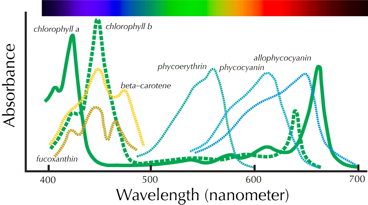
So far, you have had an opportunity to explore the nature of light and its fates in intact photosynthetic organs (leaves) and delved deeper into the architecture of the photosynthetic apparatus within the cell and as an isolated chloroplast. In this lab, you will explore the biochemical properties of the pigments within the chloroplast: chlorophylls and other pigments that capture the energy of light. Specifically, you will characterize the absorption spectra of chloroplasts and isolated pigments. The lab is open ended, in the sense that you may select photosynthetic species besides spinach. Algae (Chara and Eremosphaerea) will be available, as will plants that are growing in the greenhouse. When you select the organisms you wish to examine, the process is exploratory (Do different organisms have different pigments or not?), but you may also approach your selection with possible hypotheses in mind. Do differences occur in unusual leaves (for example with variegated coloration) or in organisms that are clearly very unrelated in evolutionary time? To assist you in your comparisons, you will be provided with protocols that enrich for particular types of pigments: chlorophylls, and carotenes. These will be compared with the absorption spectra of chloroplasts.
| Figure 1. Absorbance Workstation |
 |
Chloroplast Isolation
The chloroplast isolation is the same as in Lab 02 [http://biologywiki.apps01.yorku.ca/index.php?title=Main_Page/BIOL_4160/Visualizing_the_Photosynthetic_Apparatus], using the common STK (sucrose/tricine/KCl). The major modification is that you will use much smaller quantities of leaves (10 gm with 20 ml of STK) and homogenize with a mortar and pestle. You should have the opportunity to compare chloroplasts from completely different phylogenetic clades (higher plants and algae).
STK (pre-chilled on ice):
- Sucrose (FW 342.3) 0.6 M
- Tricine (FW 179.2) 0.05 M
- KCl (FW 74.55) 0.02 M)
Other materials: Spinach, Mortar and pestle (pre-chilled on ice), Algal cultures, Glass homogenizer (pre-chilled on ice), Cheesecloth (to filter the homogenates), Centrifuge and centrifuge tubes (to pellet the chloroplasts), and Miscellany (beakers, cuvettes, No. 1 filter paper etc.)
Don't forget that pre-chilling is important! It minimizes chloroplast deterioration due to proteolytic and lipolytic activity.
Pigment Isolation
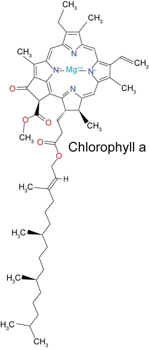
Chlorophylls
The standard extraction solvent for chlorophylls is ice-chilled acetone:water (80:20 by volume). In its simplest form, a small amount of tissues can be homogenized with a mortar and pestle in a small volume of the solvent: For example, 10 grams of plant material and 10 ml of the solvent. The homogenate is filtered through a relatively coarse filter paper (Whatman No. 1), and used as is to measure the absorbance spectrum. In land plants, the two major chlorophylls are chl a and chl b. These have different absorbance spectra, and can be distinguished in a mix by the absorbance at specific wavelengths. Further purification is necessary to separate the two pigments, something we will not do in this lab.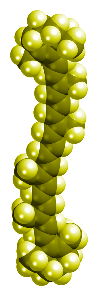
Carotenes
For carotenes, it is not possible to extract them selectively in tissues that contain chlorophylls, resulting in a mixture 'contaminated' by chlorophylls. Carotenes are more hydrophobic than chlorophylls, so partial separation is possible using a more hydrophobic mix of solvents. We will use ice-chilled petroleum ether. The homogenization is done similarly to chlorophyll extraction, using a mortar and pestle, but use 2 grams of plant material and 10 ml of the solvent. The homogenate is filtered through a relatively coarse filter paper (Whatman No. 1), and used as is to measure the absorbance spectrum. Further purification to remove the chlorophylls is both complicated and time consuming (see Discussion page). We won't do this. Instead, you should be able to distinguish the carotene spectrum from contamination by residual chlorophylls by comparing the spectra you obtain with the spectra of the acetone:water chlorophyll extracts. For all three samples (chloroplasts, acetone:water extracted chlorophylls and petroleum ether extracted carotenes) you may need to dilute to obtain a clear spectrum. This may require some trial and error on your part --the rule of thumb is a concentration dilute enough so that you can clearly see through the solution in a testtube. Don't forget to stir your chloroplast suspension. The absorbance spectra should be similar to the spectra shown in the Introduction (chloroplasts are likely to look different, why?).Absorbance Spectra Measurements --Setup
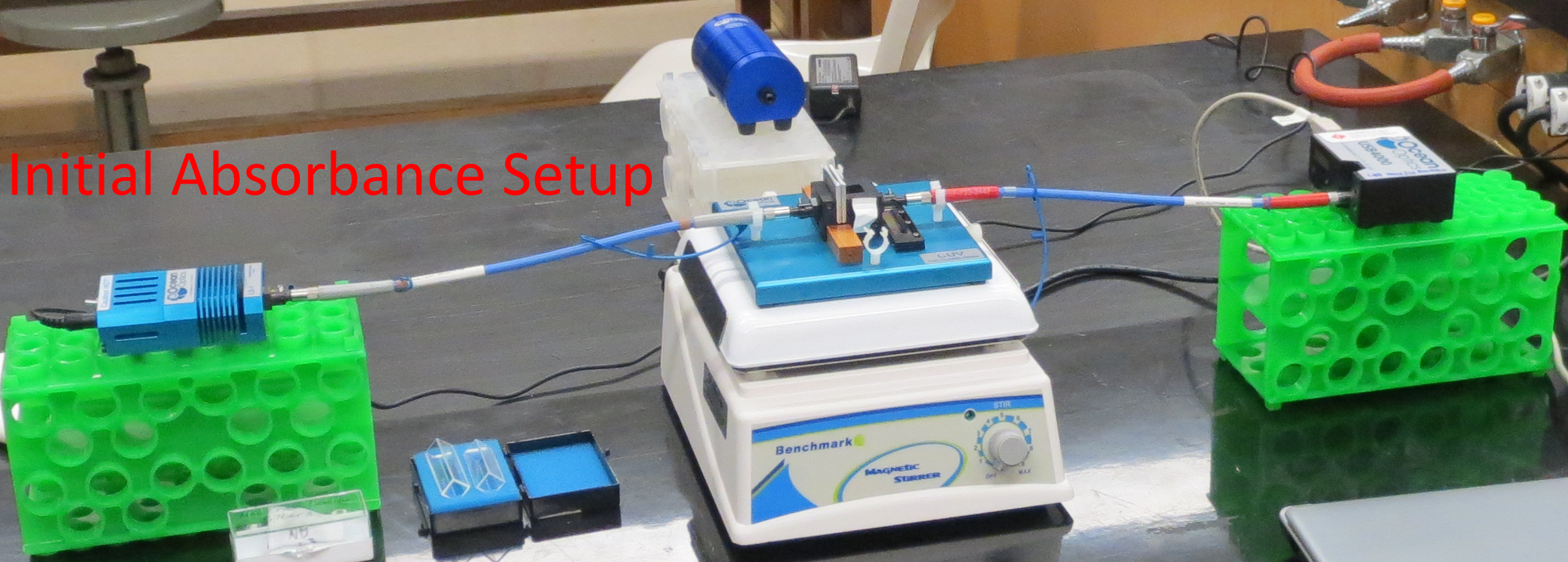
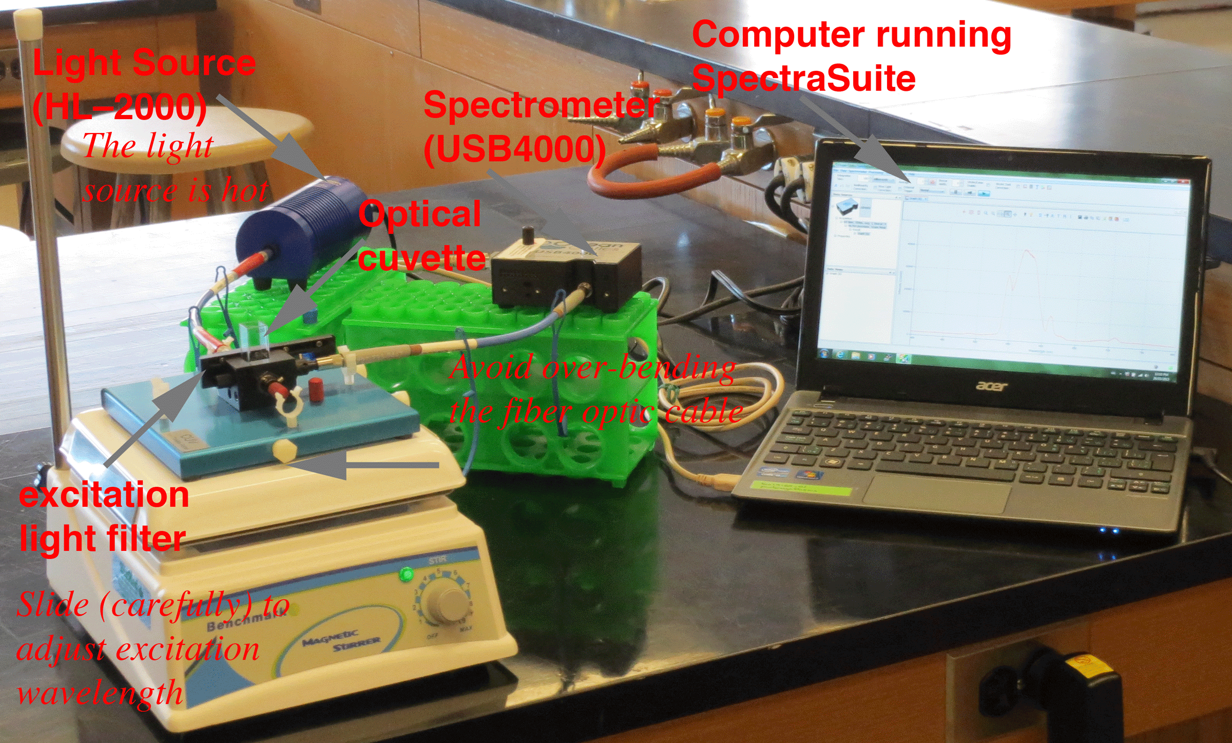
| Figure 2. Absorbance Setup (showing all components). |
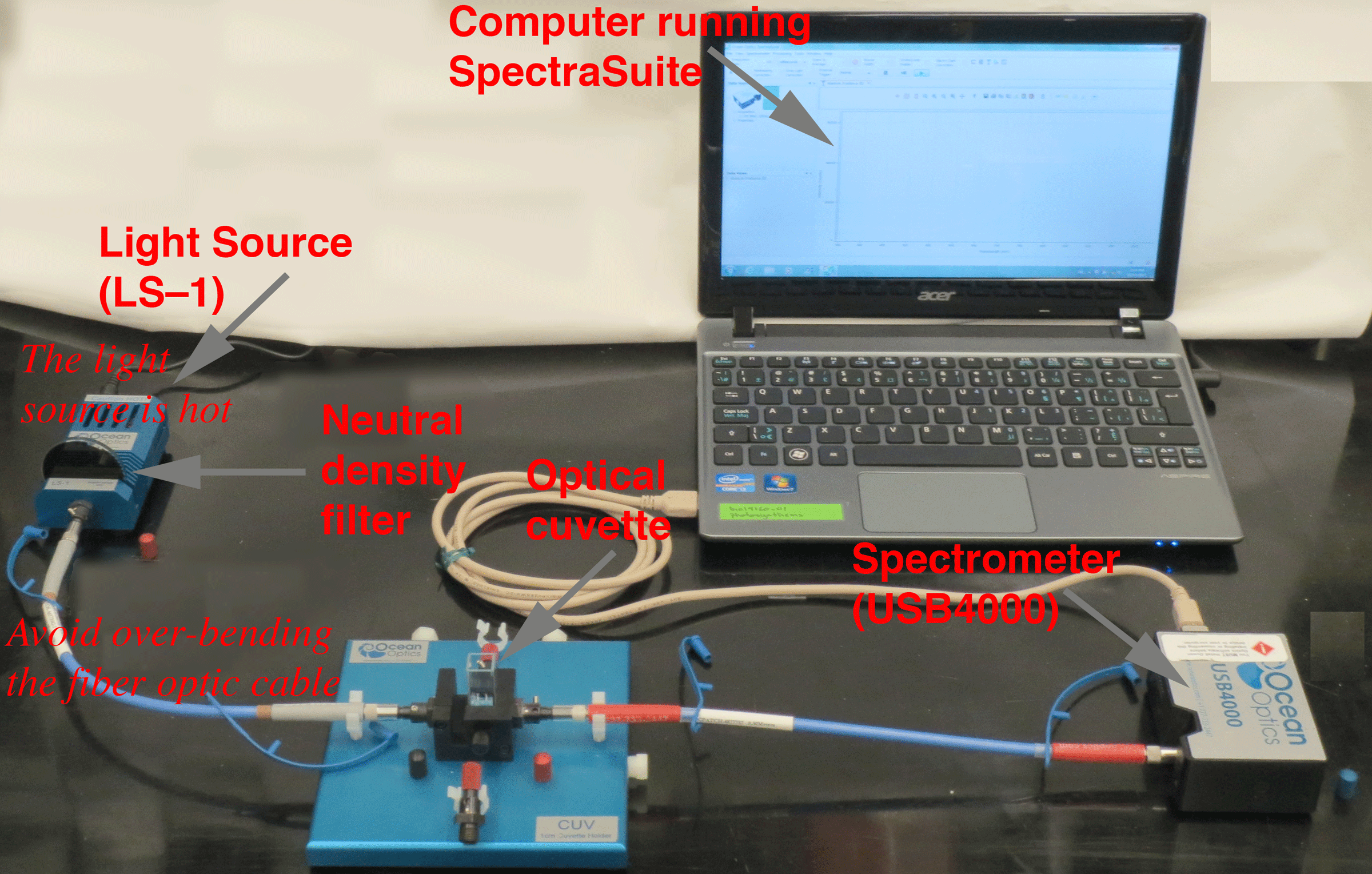 |
The instrumentation setup (Figure 2) includes the computer running the SpectraSuite software. The computer is connected to the spectrometer via a USB cable. The fiber optic lead from the cuvette holder is connected to the spectrometer. The other is connected to the light source (a tungsten halogen lamp). The light source can be hot, so be careful touching the housing. The fiber optic cables can be damaged by over-bending, so be gentle. Note that it is necessary to use a neutral density filter (OD 3) --to attenuate the light intensity entering the spectrometer. Not shown --but also very important-- is a 3.5% cupric sulfate heat shield. This fits into the slot next to the cuvette on the cuvette holder. The cupric sulfate solution attenuates infrared radiation from the lamp to maximize the absorbance signals in the visible light range.
For your chloroplast absorbance measurements, the chloroplast suspension in the cuvette must be stirred. For pigments isolated in solvents, stirring is not required.
Absorbance Spectra Measurements --Calibration
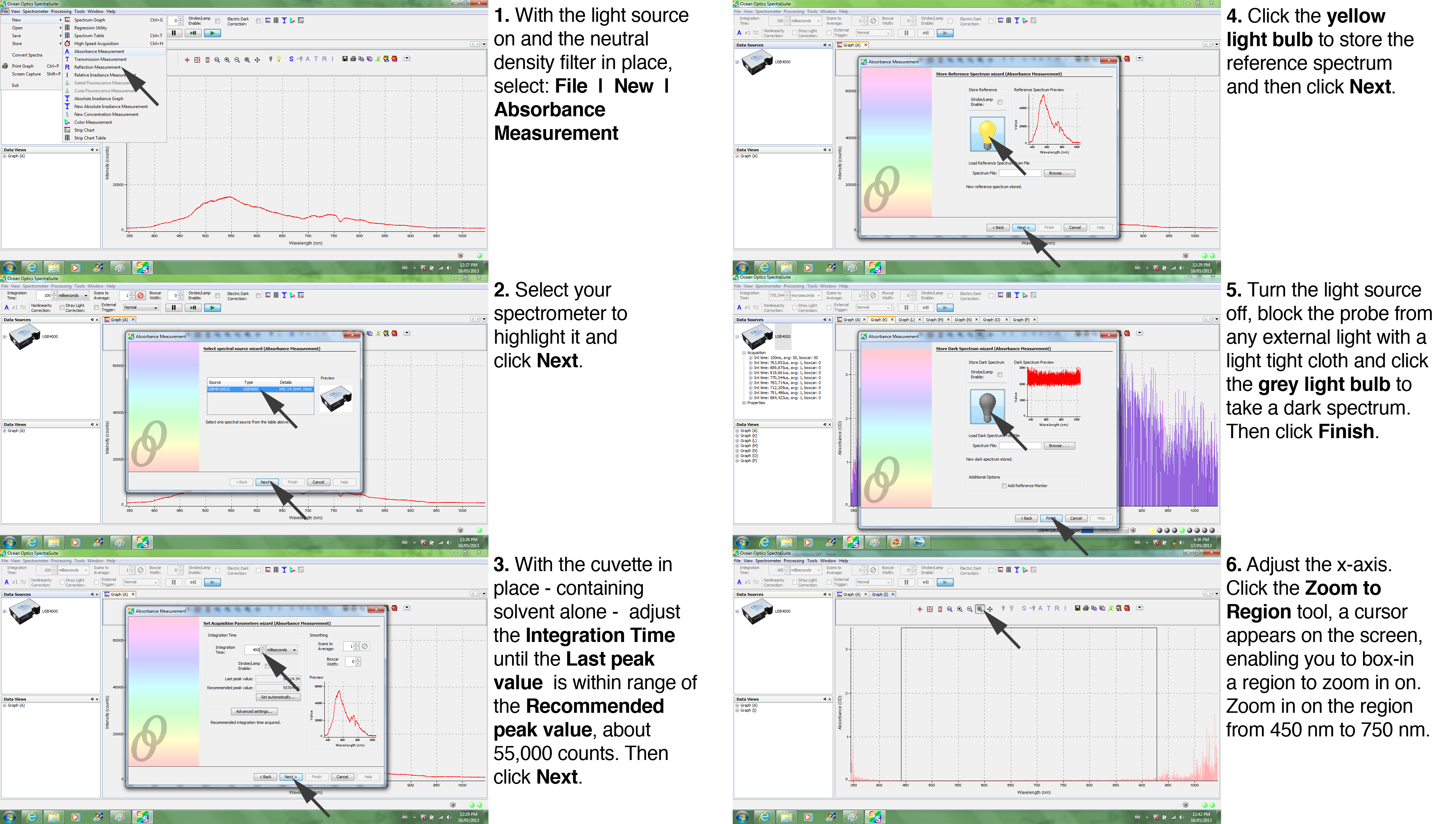
Calibration is absolutely crucial --to account for the spectral output of the tungsten halogen lamp. The calibration steps are shown below in Figure 3. First, select File | New | Absorbance Measurement. Highlight the spectrometer and click Next. Then, with the light source on (be sure the neutral density filter is in place), adjust the Integration Time until the Last peak value is within range of the Recommended peak value, about 55,000 (this doesn't have to be exact, just in the range: 45,000 is fine, 60,000 is too much). This ensures that the signal does not 'clip' at a level higher than the maximum measurable by the spectrometer. In the next steps, you record the spectra with the light bulb still 'on', then with the light bulb 'off.' For the latter, you need to turn off the light source (the switch is on the back of the LS-1 unit) and shade the probe from stray light with a light tight cloth. First, with the light still on click the yellow light bulb to store the reference spectrum and click Next. Turn off the light source to take a dark spectrum. The graph appears on the right side of the screen. Click the grey light bulb then Finish. Lastly, adjust the scaling on the x-axis (wavelength) by zooming in on the region of interest, 450 nm to 750 nm. You are now ready to measure the absorbance spectra of the pigments you isolated.
| Figure 3. Absorbance Calibration Tutorial |
 |
Carotenoids
Literature searching for techniques to isolate carotenoids selectively revealed a deep historical pedigree. The original method came from work by Willstatter and Stoll, who were pioneers in the extraction of plant pigments. Their technique, and more recent modifications are described in a 1941 article by Walter J Peterson (Recent Developments in Methods for Determining Carotene. Industrial and Engineering Chemistry-Analytical Edition. 13:212-216). Much of the literature focuses on carotenes as a vitamin; a common starting material for analysis is forage for cattle (alfalfa). What all the methods have in common is extraction with various solvents (acetone, ether, and petroleum ether are examples), followed by removal of the chlorophylls (and other pigments) by treatment with alkaline (by KOH addition) methanol (or ethanol). For example, after extraction of carotenes by petroleum ether, removal of residual chlorophyll can be performed by shaking the petroleum ether extract with 25% KOH in methanol, and removing the methanol (containing chlorophyll).(Russell WC, Taylor MW, Chichester DF (1935) Colorimetric determination of carotene in plant tissue. Plant Physiology 10:325-340.). Another method is to reflux the carotenoids with barium hydroxide (Petering HG, Morgal PW and EJ Miller (1940) Isolation of carotene from green plant tissue. Industrial and Engineering Chemistry. 32:1407-1412).
Subsequent purification can be done with thin layer chromatography or column chromatography. If the focus of these lab exercises was more 'chemical', the ideal technique would be preparative thin layer chromatography. Preparative means a large quantity of the pigments --extracted with acetone-- would be streaked at the bottom of a large plate. After pigment separation in a developing tank using petroleum ether, each band could be scraped off and re-dissolved in a quantity large enough for spectral measurements. But this takes a long time. For our purposes, we need something simple, that allows students to visualize the carotenes in a reasonable period of time.
Fluorescence and Reaction Centers
Introduction to Fluorescence Spectroscopy
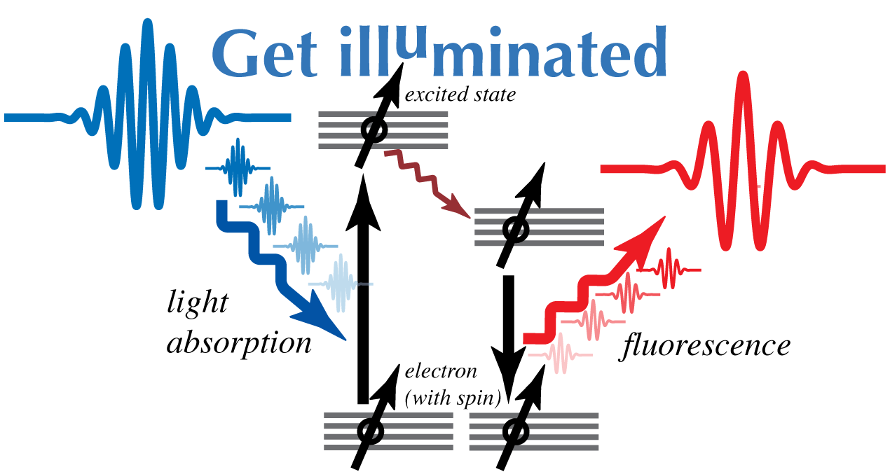
Fluorescence is an example of luminescence --described in your first lab as the emission of light when 'excited' electrons fall to a lower energy. Usually, the electron becomes excited in the first place due to the absorption of a photon (Figure 1)
In the case of chlorophyll, there are two major orbital levels (a high energy orbital equivalent to a 'blue' photon [about 400 nm] and a low energy orbital equivalent to a 'red' photon [about 700 nm]). Normally, excitation to the high energy orbital is the result of the absorption of a 'blue' photon. The wavelength of the fluorescence is longer because some of the energy is lost through radiation-less relaxation, resulting in red fluorescence.
In chloroplasts under physiological conditions, the fluorescent light emitted by chlorophyll (Chl) is associated almost entirely with the photosystem II reaction center. There are two types of fluorescence: prompt and delayed. The prompt fluorescence decays in about 10-8 sec and arises from relaxation of the excited state of antenna Chl (Chl*):
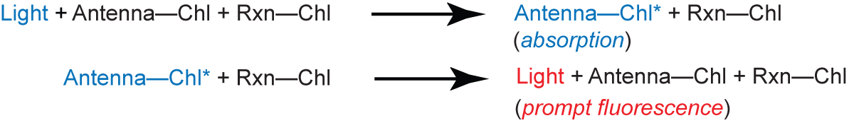
Note that the reaction center (Rxn-Chl) is never excited.
In contrast, the delayed fluorescence arises from reversal of photochemistry at the reaction center:
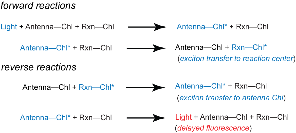
The prompt fluorescence is about 100 times more intense than the delayed fluorescence. The yield of prompt fluorescence is governed by the activity of the reaction center of photosystem II: The more efficiently the energy of the excited Chl is used for photochemistry, the less is given off by fluorescence (and vice versa). Therefore, variations in the prompt fluorescence give insight into the state of photosystem II.
The yield of delayed fluorescence is normally low because the reaction center Rxn-Chl* usually donates the excited electron to a donor (X):

The reduced donor X- infrequently supplies an electron back to the reaction center to produce the excited state Rxn-Chl*.
The intensity of delayed fluorescence is governed by several factors.
First, any factor that alters the yield of prompt fluorescence will similarly affect the yield of delayed fluorescence.
In addition, the delayed fluorescence depends on the concentration of X- that can react to give Rxn-Chl*. If secondary electron transfer reactions, for example, the donation of an electron to the Rxn-Chl+
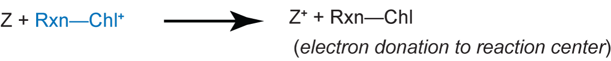
are prevented or caused to go in reverse, the concentration of Rxn-Chl+ + X- increases and the delayed fluorescence becomes more intense because re-donation of the electron to Rxn-Chl+ is more likely.
A final factor is the 'energy state' for photophosphorylation (light-driven ATP synthesis), which is probably a combination of the proton gradient and electric potential across the thylakoid membrane. When the 'energy state' is high, it increases the delayed light emission, probably by raising the energy of the reduced primary acceptor X-. This would increase the probability of the energy-requiring reaction
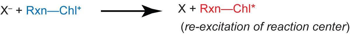
and subsequent delayed fluorescence. This effect is especially strong because it acts exponentially: If the necessary increment of energy is ∆E, the probability of the reaction is proportional to the Boltzmann factor exp(∆E/kT).
There may be more subtle causes for changes in delayed fluorescence, since many factors could affect the energy of the reduced primary acceptor, reduction of Chl+, and indeed, prompt fluorescence. All told, the magnitude of prompt and delayed fluorescence provides insight into multiple and complex processes in photosynthesis, and, the effects of particular agents in electron transport and/or phosphorylation.
As one example, if a chemical treatment (for example, DCMU which blocks downstream electron transfer) causes a sudden increase in the intensity of fluorescence, it can be mistaken for a case of chemiluminescence.
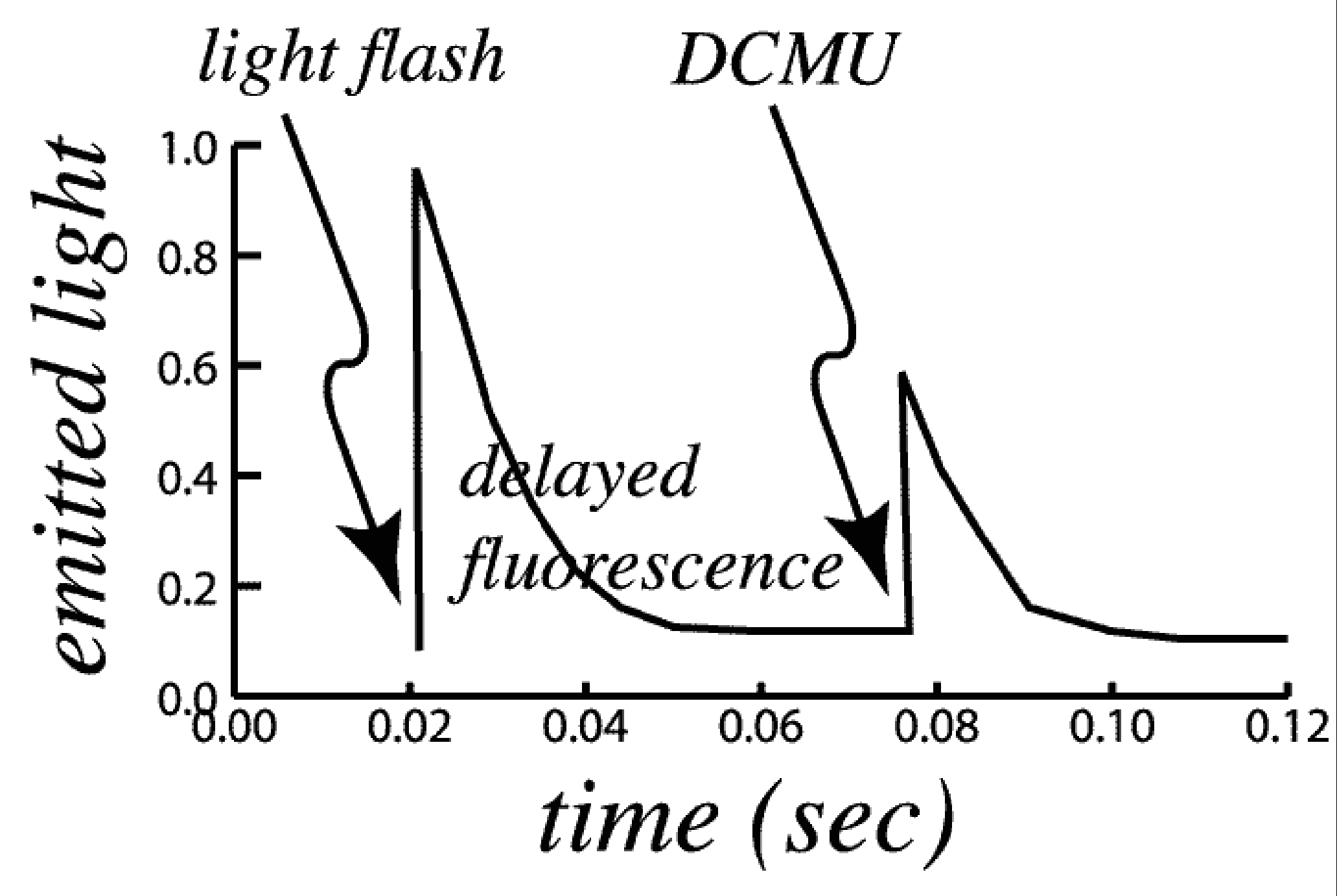 |
Figure 1. Two aspects of delayed fluorescence are shown in the figure. Delayed fluorescence reveals the reversal of the Chl•X- state. DCMU blocks electron transfer downstream of the photochemical Chl•X- state, resulting in even more release of exciton energy as fluorescence from the reaction centers. |
Two aspects of delayed fluorescence are shown in the figure. Delayed fluorescence reveals the reversal of the Rxn-Chl+ + X- state. DCMU blocks electron transfer downstream of the photochemical Rxn-Chl+ + X- state, resulting in even more release of exciton energy as fluorescence from the reaction centers.
When the reaction center is in the state Rxn-Chl+ + X-, it is unable to use light energy to perform photochemistry until X- has released its electron to a chain of electron carriers leading to photosystem I and reverted to the non-reduced X. The unused light energy may be emitted as fluorescence. Thus the intensity of delayed fluorescence is high when the reaction center is in the Rxn-Chl+ + X- state, and low when the reaction center is in the state Rxn-Chl + X. DCMU prevents electrons from leaving X-, and also causes the return of electrons from secondary acceptors to X. Thus, DCMU causes a high intensity of prompt fluorescence and increases the intensity of delayed fluorescence immediately after it is added.
Summary
Fluorescence is readily separated into fast fluorescence (prompt) and delayed fluorescence. Both represent a loss of light energy for use in photosynthesis, and therefore provide a metric for photosynthetic efficiency. Prompt fluorescence represents the immediate loss of the absorbed energy, from excitons that were never able to reach the reaction center. Delayed fluorescence is more complicated. It is the backflow of excitons from the reaction center, or even the redox reactions that occur as a consequence of charge separation at the reaction center. Both prompt and delayed fluorescence provide insight into the state of the photosynthetic process and are therefore important diagnostic tools for the photosynthesis researcher.
In these exercises, we will examine prompt and delayed fluorescence in isolated cells, chloroplasts and chlorophyll. We will do so using a fluorescence spectrometer (fluorometer).
How Fluorescence Spectroscopy Works
| Figure 2. Light Scattering |
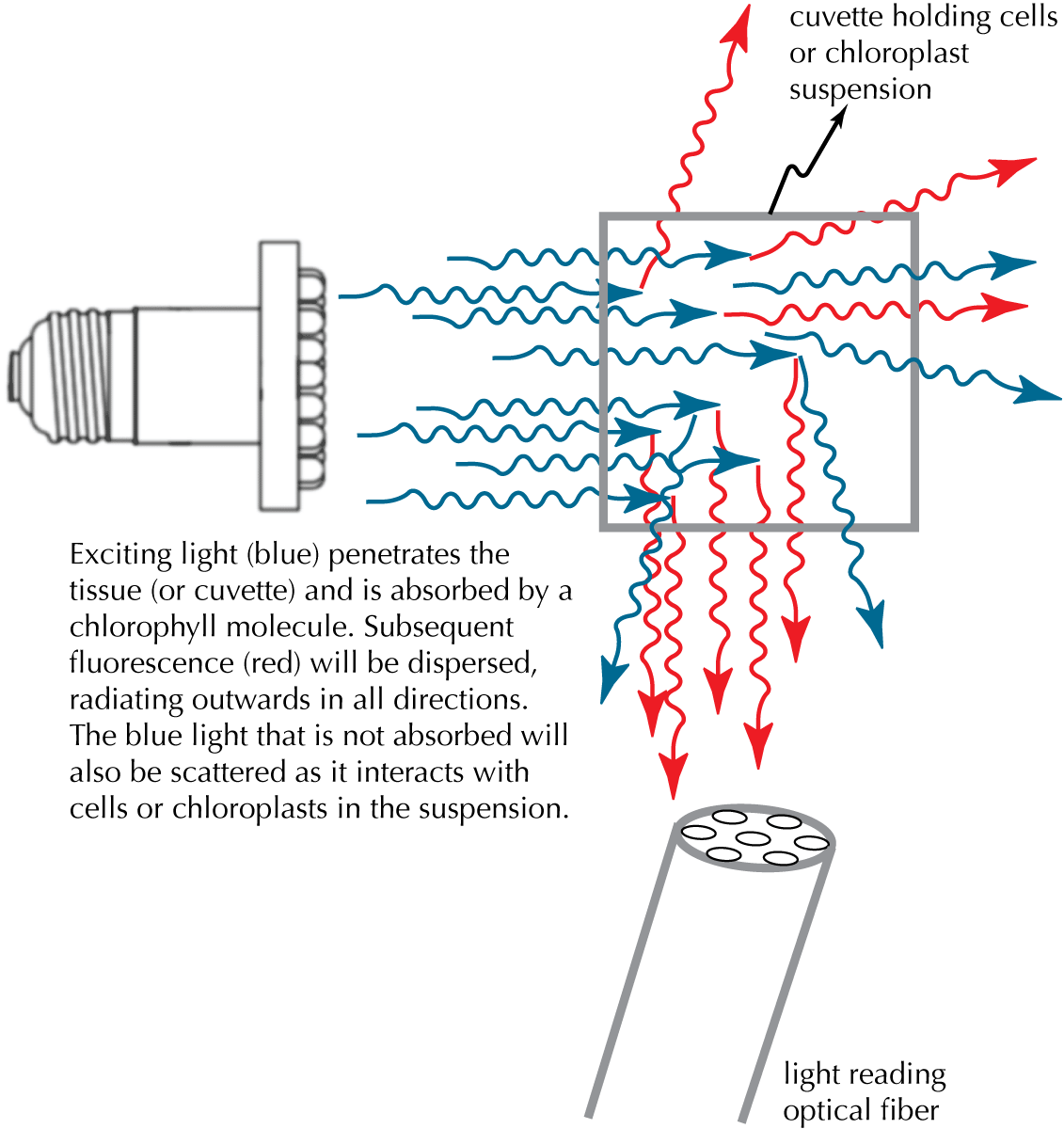 |
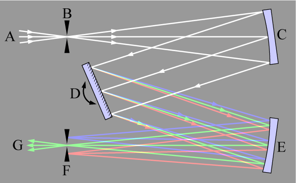 |
Figure 3. Light (A) is focused onto an entrance slit (B) and is collimated by a curved mirror (C). The collimated beam is diffracted from a rotatable grating (D) and the dispersed beam re-focussed by a second mirror (E) at the exit slit (F). Each wavelength of light is focussed to a different position at the slit, and the wavelength which is transmitted through the slit (G) depends on the rotation angle of the grating. From Wikipedia: en.wikipedia.org/wiki/Monochromator |
The system we will be using is different, utilizing recent advances in light-sensing systems. For excitation, a linear interference filter provides specific wavelengths of light. For emission, the light from the diffraction gradient impinges on a linear CCD detector, so that all wavelengths of emitted light are measured simultaneously. A schematic is shown in Figure 4.
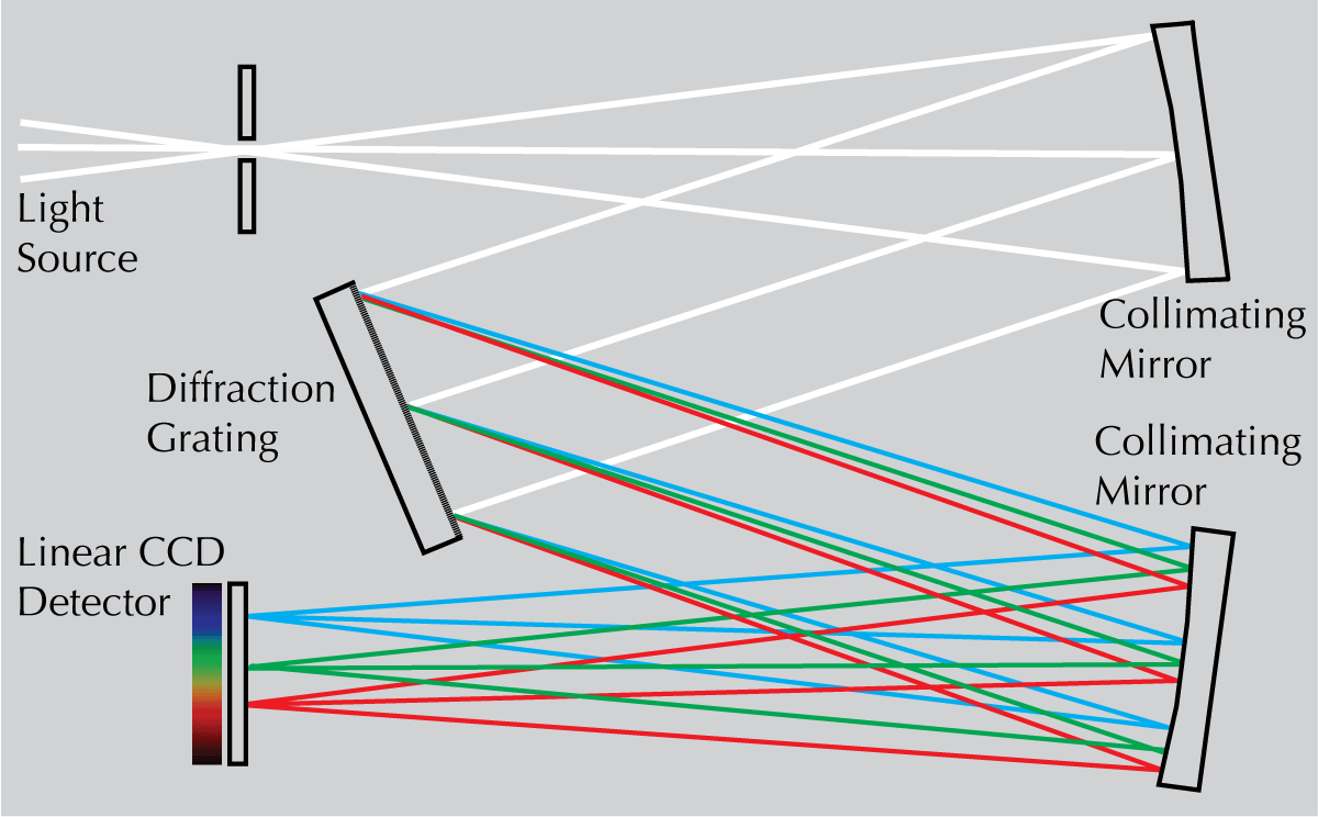 |
Figure 4. Unlike the monochromator, the light does not exit through a slit (thereby selecting for a narrow range of wavelengths), but instead impinges on a CCD light detector, so that all the wavelengths are collected simultaneously. This means that scattered light will also be seen, so that a light scattering control (using dilute milk) is necessary. |
A general spectra for absorbance and fluorescence of chlorophyll is shown below:
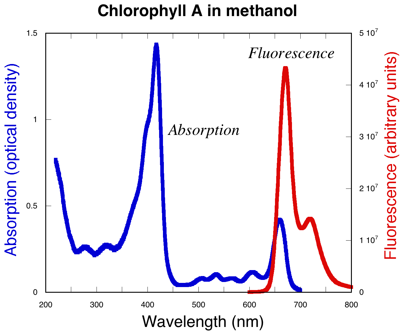 |
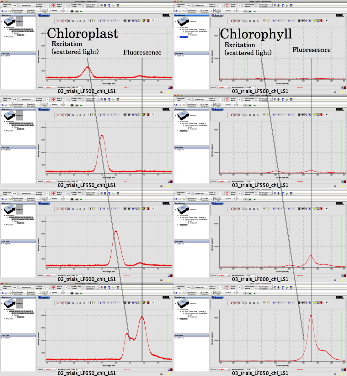
The absorbance (excitation) and fluorescence (emission) wavelengths of chlorophyll vary depending upon the solvent in which the chlorophyll is dissolved. So it is necessary to measure excitation and emission spectra for chlorophyll in the chloroplast using the fluorometer. Prompt fluorescence will be measured by measuring the emitted light during excitation. Delayed fluorescence is measured by irradiating the chloroplast suspension at high light intensity. Then, the chloroplast suspension is injected into the cuvette. Measure only the emitted light (the excitation light must be turned off) to observe the delayed fluorescence.
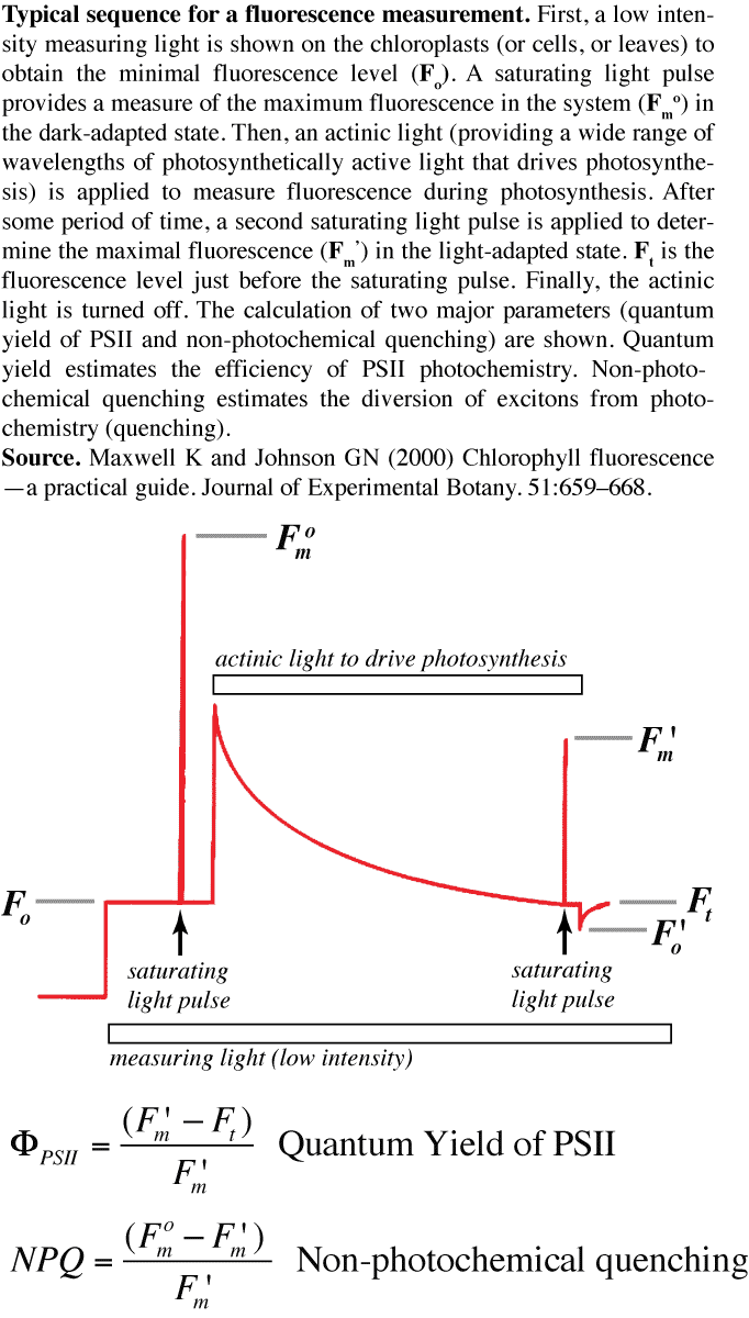
As should be clear from the introductory remarks, fluorescence can be used as a diagnostic for the 'state' of photosynthesis. This is a very common technique in photosynthesis research, because it can be used in the field (using special --and expensive-- instrumentation). Kate Maxwell and Giles Johnson wrote a primer on chlorophyll fluorescence which gives a good flavour of how fluorescence is used as a diagnostic: Maxwell K and Johnson GN (2000) Chlorophyll fluorescence --a practical guide. Journal of Experimental Botany. 51:659--668. http://jxb.oxfordjournals.org/content/51/345/659.long. The figure shows how these measurements are made, and some of the major calculations.
Lab 04 Determining Excitation and Emission Spectra
General Objective
To measure and compare the absorbance and emission spectra of isolated chloroplasts with the absorbance and emission spectra of the chlorophyll pigments.
Chloroplast Isolation
Solutions
STK (pre-chilled on ice):
- Sucrose (FW 342.3) 0.6 M
- Tricine (FW 179.2) 0.05 M (Tricine buffer has a pK of 8.15. The pH of the media is adjusted to 7.5 with KOH/HCl, as required.)
- KCl (FW 74.55) 0.02 M (mimics the ionic environment of the cytoplasm)
TK (prechilled on ice):
- As above, without sucrose (used to dilute your stock chloroplast suspensions)
Ac/W:
- 80% acetone, 20% H2O (to isolate chlorophyll pigments)
Milk (dilute):
- a small aliquot of whole milk in H2O (1/100) (the fat globules are effective at scattering light)
Other materials: Spinach, Mortar and pestle (pre-chilled on ice), Algal cultures, Glass homogenizer (pre-chilled on ice), Cheesecloth (to filter the homogenates), Centrifuge and centrifuge tubes (to pellet the chloroplasts), and Miscellany (beakers, cuvettes, No. 1 filter paper etc.)
Isolation Procedure
Rinse spinach in tap water, remove midribs with scissors (or razor, but scissors are easier and faster) and cut the remaining tissue into pieces of about 2 cm width and length.
About 10 grams of spinach should be placed in a pre-chilled mortar and pestle with 50-100 ml of pre-chilled STK. Grind in a mortar and pestle, ensuring that all leaves are compacted down and effectively homogenized. The homogenate is poured through three layers of cheesecloth into a pre-chilled beaker in ice. The cheesecloth can be squeezed gently to release more chloroplasts. Centrifuge for 1-2 min at 500 X g to spin down debris. The supernatant should be centrifuged for 10 min at 10,000 X g to spin down the chloroplast into a pellet. Decant the supernatant and gently disperse the pellet into about 5 ml of STK. Keep the chloroplast suspension on ice.
If algal cells are provided... when you harvest the algal cultures, the technique for isolating chloroplasts will vary depending on the type of algae. If you are provided with Chara australis, it is as simple as cutting one end of the internode cell (with small scissors) and squeezing the cell sap (with chloroplasts) onto a microscope slide. If you are provided with Eremosphaera viridis, the large cells need to be broken apart. This is done with a glass mortar and pestle. The cells are decanted from the culture flask into a 50 ml disposable centrifuge tube, allowed to settle (this will take less than 5 minutes at "1 X g"). The supernatent (culture media) is carefully poured off (into the sink) and the cells re-suspended in STK. Then, they are poured into the glass homogenizer. The plunger is pushed to the bottom while twisting it. This is repeated 4 times, at which point the cells will have been disrupted, releasing the chloroplasts. The homogenate is filtered through multiple layers of cheesecloth, and the filtrate (chloroplast rich) is used as is for microscope visualization.
When performing fluorescence measurements, the amount of fluorescence will depend upon the concentration of the chloroplasts. So, it is important to ensure the same amount of chloroplasts is used for all measurements. Normally, the chlorophyll concentration is used to standardize chloroplast concentrations. Note that the spectrometer configuration for absorbance measurements is different from the configuration for fluorescence.
 So, do your absorbance measurements first, then re-configure the setup for fluorescence. In SpectraSuite, you can select particular wavelengths to obtain the absorbance (shown at the bottom of the graph). For fluorescence, there is no calibration required (you are measuring relative intensities). The integration time can be adjusted to get a good signal.
Standardizing Chloroplast Concentration
| Absorbance (sometimes called optical density, abbreviated OD) is a logarithmic measure of light absorption: If light of an intensity Io enters the sample and a lesser intensity I exits: A = log10(Io/I). This logarithmic measure has the virtue that it is proportional to the concentration of light-absorbing material in the sample. In a laboratory, a path length through the sample of 1 cm is the common convention. Thus, your cuvettes are 1 cm in width. In some research fields, absorbance is defined as the natural logarithm of the ratio Io/I (A = ln((Io/I), but OD (OD = log10(Io/I) is the more common measure, and what is measured by your Ocean Optics spectrometer. An additional source of confusion is that the equation is sometimes shown in the equivalent form OD = -log10(I/Io). Because it's easy to lose the negative sign, I prefer log10(Io/I). |
Chl a = 12.7 (OD662) - 2.7 (OD645) (micrograms / ml)
Chl b = 23.0 (OD645) - 4.7 (OD662) (micrograms / ml)
Calculate the concentrations of chlorophylls in the stock suspension based upon the dilution factor you used to make the Ac/W extract. For example, if you used 0.05 ml of suspension (in 5.0 ml of Ac/W), the dilution factor is 5.05 / 0.05, or 100-fold. Adjust the volume of the chloroplast suspension to a concentration of about 0.1 to 0.5 mg/ml Chl using STK. A sample calculation can be found at the end of the lab exercise [http://biologywiki.apps01.yorku.ca/index.php?title=Main_Page/BIOL_4160/Determining_Excitation_and_Emission_Spectra#Calculation_of_Chlorophyll_Concentration]. Be sure to save your chlorophyll pigments (on ice) for measurements of excitation/emission spectra of pigments (to compare with chloroplasts). For most experiments, the stock suspension of chloroplasts will be diluted into TK solution to a final density of 10 micrograms/ml Chl. However, chloroplasts should always be stored concentrated since this improves their viability outside of their native environment.
Fluorescence Spectra Measurements --Setup
| Figure 1. Fluorescence Setup |
 |
The instrumentation setup includes the computer running the SpectraSuite software (Figure 1). The computer is connected to the spectrometer via a USB cable. One of the fiber optic leads is connected to the spectrometer. The other is connected to the light source (a high intensity tungsten halogen lamp). The light source can be hot, so be careful touching the housing. The fiber optic cables can be damaged by overbending, so be gentle. The two fiber optic leads are connected at the cuvette holder at right angles. The wavelength of the excitation light is adjusted by sliding the filter carefully --the scattered light peak will be observable as part of the SpectraSuite spectrum.
There are some crucial points to bear in mind when you setup the apparatus.
- Make sure you shield the cuvette from extraneous illumination. Otherwise, scattered light from the fluorescence lighting will 'contaminate your spectra. You should be able to determine whether this is a problem by monitoring the spectra.
- Be careful when sliding the excitation filter to adjust the excitation wavelength. This is a very expensive interference filter, so two hands are better than one. Let your lab mate collect the spectra on the computer, as required).
Determining Excitation and Emission Spectra
| Figure 2. Fluorescence Scans. Here are examples of fluorescence scans chloroplasts and acetone/water extracted chlorophyll to give you an idea about the kind of scans you will see with your preparations. Note that chloroplasts scatter light much more than chlorophyll does. Why? |
 |
Calculation of Chlorophyll Concentration
The following example is fictitious, but shows you how to calculate chlorophyll concentration and dilution factors. Take 0.05 ml of your chloroplast suspension (ensuring it is well-mixed before drawing the aliquot) and add to 5 ml of Ac/W. In the spectrometer, you measure blank (Ac/W alone) values of 'zero', and sample absorbances of:
OD662: 0.5
OD645: 0.2
Filling in the blanks of the equations
| Chl a = 12.7 (OD662) - 2.7 (OD645) (micrograms / ml) | Chl a = (12.7)(0.5) - (2.7)(0.2) = 5.81 micrograms/ml |
| Chl b = 23.0 (OD645) - 4.7 (OD662) (micrograms / ml) | Chl b = (23.0)(0.2) - (4.7)(0.5) = 2.25 micrograms/ml |
| Total chlorophyll is | 8.06 micrograms/ml, or 0.00806 mg/ml |
Since the dilution was 100-fold, your suspension chlorophyll is 0.806 mg/ml
Now, suppose you want a final chlorophyll suspension of 0.05 mg/ml in a total volume of 5 ml (for fluorescence measurements):
(X/5)*(0.806) = 0.05 (in units of mg/ml)
The algebra..... X = (5)(0.05)/0.806 = 0.31 ml
So..... add 0.31 ml of suspension and 4.7 ml of your suspension medium to reach 0.05 mg/ml
If you want a final chlorophyll suspension of 0.50 mg/ml in a total volume of 5 ml (for oxygen electrode measurements):
X = (5)(0.5)/0.806 = 3.1 ml. So add 3.1 ml of your suspension with 1.9 ml of suspension medium.
Keep your concentrated chloroplast suspension (on ice)! As noted, high concentrations improve stability.
Reference for Calculating Chlorophyll Concentrations
The reference for calculating chlorophyll concentrations is an article by Daniel I. Arnon from 1949:
- Arnon, DI (1949) Copper enzymes in isolated chloroplasts. Polyphenoloxidase from Beta vulgaris. Plant Physiology 24(1):1-15.
Lab 05 Physiology of Fluorescence
Fluorescence and the Reaction Centers
Having measured the excitation and emission spectra for chloroplasts, you will now be able to explore the relation between fluorescence and the physiological function of the reaction center. As explained in the introduction to the fluorescence labs [http://biologywiki.apps01.yorku.ca/index.php?title=Main_Page/BIOL_4160/Fluorescence_and_Reaction_Centers], treatments that perturb the reaction centers will have an effect on both prompt and delayed fluorescence.
Visualizing delayed fluorescence is very difficult because the photon emissions are low, at the limits of the sensitivity of the spectrometer. So, in this exercise, you should measure prompt fluorescence first (to ensure you will get results!). Then, if time permits, you can try to visualize the delayed fluorescence.
Prompt Fluorescence
For prompt fluorescence, setup your chloroplasts as in the excitation/emission measurements. Select an excitation wavelength (by moving the linear bandpass filter) that provides you with a strong fluorescence signal. Then, add the reagents as described below.
Stock solutions
Electron Transport Block- 0.01 M DCMU (diuron) (3-(3', 4' - dichlorphenyl) - 1,1 - dimethylurea) (FW 233.1) in ethanol [blocks electron transport]
- sodium dithionite (10 mg/ml) [strong reductant]
- 0.25 M succinic acid (FW 118.1) [strong acid]
- 1.2 M Tris (base) (FW 121.4) [strong base]
DCMU injection
Prepare the DCMU by adding 0.1 ml of 0.01 M DCMU (ethanol solution) to 0.9 ml of dH2O, and mix well. After recording the fluorescence spectrum of the chloroplasts in the cuvette, add 0.2 ml of the DCMU to the chloroplast suspension in the cuvette. To assure good mixing, ensure that the stir bar is working. Record the effect of DCMU on prompt fluorescence.Dithionite injection
Dissolve 10 mg of Na-dithionite (a strong reductant) into 1 ml of dH2O, mix well. Add 0.2 ml to a new chloroplast suspension in the cuvette. Ensure that the stir bar is working to assure good mixing. Record the effect of dithionite on prompt fluorescence.Acid-base transition
First, add 0.2 ml of 0.25 M succinic acid to the cuvette. Then add a new chloroplast suspension. The chloroplasts should be at a pH of about 4.5. Record the prompt fluorescence. Then inject 0.2 ml of 1.2 M Tris base into the cuvette. This will cause the pH to increase to about 8.5, and generate a pH gradient across the thylakoid membranes.Delayed Fluorescence
To measure delayed fluorescence, the chloroplasts are first irradiated under bright light, then injected into the cuvette in the fluorometer. Please ensure the excitation light source is turned off (otherwise you will be measuring prompt fluorescence). The injection should be done quickly, to minimize the delay, but not so fast as to cause spillage. When injecting, take care to ensure that no ambient light (from the room lighting) 'leaks' into the measuring compartment (cuvette) of the fluorometer (use the white 'black-out' cloth). Monitor the emitted fluorescence over time. For these experiments, it will be necessary to increase the integration time of the spectrometer (to maximize the sensitivity) to measure the emitted light. You may also need to change the scaling on the y-axis of the spectrum graph to ensure the relatively small changes will be readily observed.
For inhibitor effects on delayed fluorescence (DCMU), the chloroplasts should be pre-irradiated prior to injection into the cuvette, and the delayed fluorescence measured prior to and after the addition of the electron transport chain blocker.
Describe and Interpret the Results.
Oxygen Electrode: Pathways of Photosynthetic Electron Transport
General Introduction
The light reactions of photosynthesis require a supply of electrons to constantly replenish the reaction center of Photosystem II. The photochemistry at the reaction center: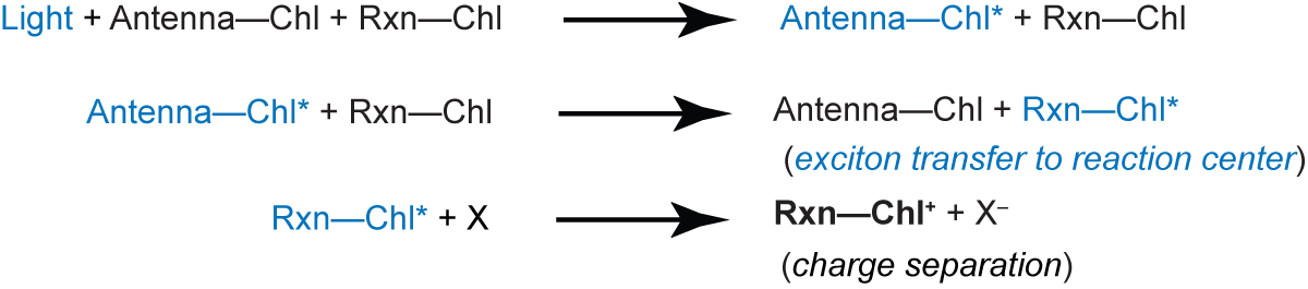
results in the creation of an oxidized chlorophyll, Chl+. Since the X- electron is donated to a secondary acceptor, the Chl+ must be reduced by a secondary reaction. In oxygenic photosynthesis, the electron source is water
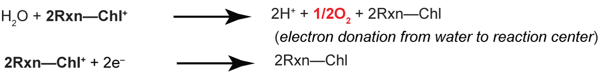
In this process, O2 is produced as an un-utilized byproduct. The oxygen electrode measures the O2 produced during photosynthesis. Like prompt and delayed fluorescence, measurements of O2 production yield a snapshot of the entire process of photosynthesis since many factors can affect the utilization of H2O in the chloroplast. In the first lab exercise, the oxygen electrode will be used to monitor effects of phosphorylation (ATP production) and uncouplers on rates of O2 evolution. From these effects, it will be possible to estimate the ratios of ATP production to electron transport (P/O ratios). Using inhibitors of electron transport, and e- donors and acceptors, Photosystem I - associated reactions can be isolated from those associated with Photosystem II. That is, it is possible to unravel the roles of the different components of the electron transport chains in photosynthesis. In the second lab exercise, you will use the oxygen electrode to explore the effect of carbon dioxide on rates of oxygen evolution, and thus demonstrate the the carbon dioxide fixation pathway is localized to the chloroplast.
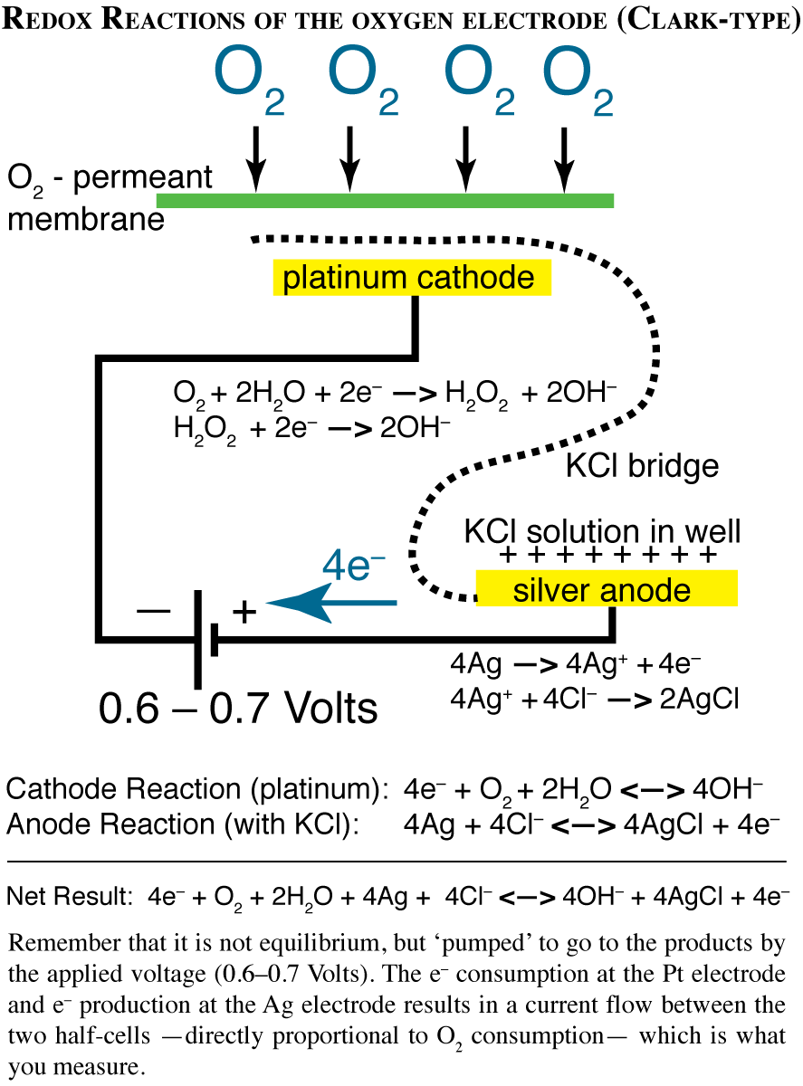
How the Clark-Type Oxygen Electrode Works
The O2 electrode consists of a silver anode and a platinum cathode electrically linked by a concentrated KCl solution. These are separated from the reaction medium by a Teflon membrane, which is permeable to O2, but little else. A small voltage is applied across the electrodes causing the platinum cathode to be negative with respect to the silver anode. When the potential is raised to 600-700 mV, O2 is reduced at the platinum cathode (to H2O) and this reduction causes a current of electrons to flow between the two electrodes. The electrical current is directly related to the amount of O2 reduced at the cathode. In a well-stirred reaction mixture, the rate of O2 reduction at the cathode is proportional to the rate of O2 diffusion across the Teflon membrane, which is proportional to the O2 concentration in the reaction medium. Changes in O2 concentration by photosynthesis (which raises the O2 concentration) or respiration (which reduces O2 concentration) can be easily determined by measuring the electrical current produced. The electronics are configured so that the output is in voltage, the output range is typically 0-1 V.
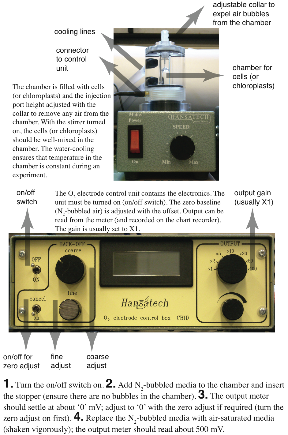
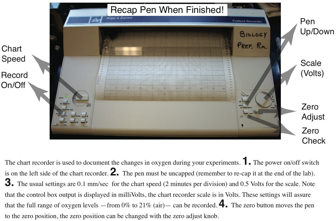
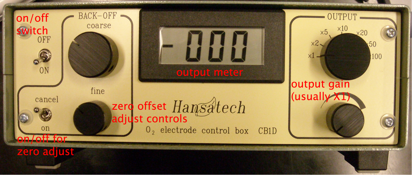 | Control Unit. The O2 electrode control unit contains the electronics. The unit must be turned on (on/off switch). The zero baseline (N2-bubbled air) is adjusted with the offset. Output can be read from the meter (and recorded on the chart recorder). The gain is usually set to X1. |
| Electrode Chamber. The chamber is filled with cells (or chloroplasts) and the injection port height adjusted with the collar to remove any air from the chamber. With the stirrer turned on, the cells (or chloroplasts) should be well-mixed in the chamber. The water-cooling ensures that temperature in the chamber is constant during an experiment. | 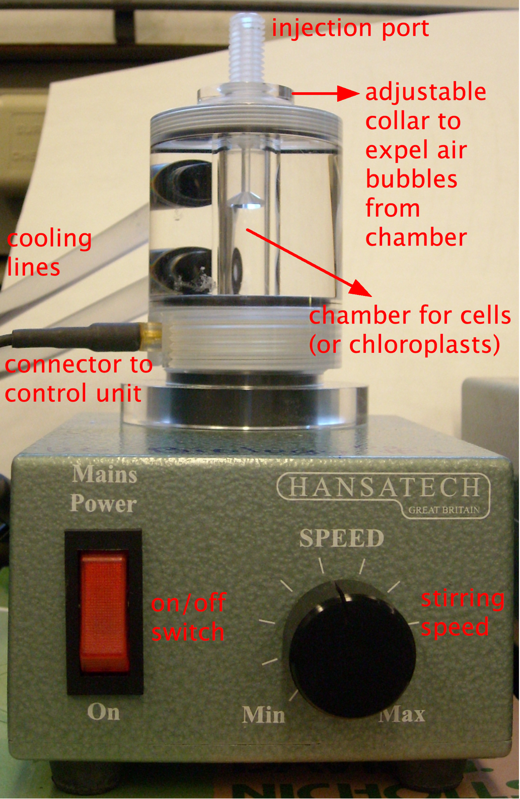 |
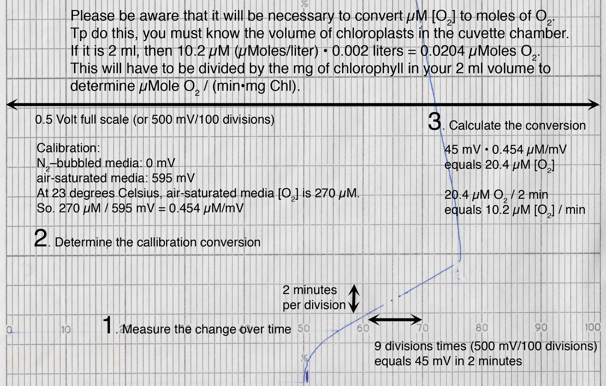
The details of recording will depend upon the instruments used. Normally, output from the Clark electrode is measured with a chart recorder, so that ∆[O2]/∆time can be quantified. The units can be uM O2 min-1 [mg Chl]-1, or nmoles O2 min-1 [mg Chl]-1 (the latter is preferred, and requires that the volume in the chamber be known). Usually, the electrode voltage is about 500 mV for air-saturated H2O.
Calibrating the Oxygen Electrode
To calibrate the oxygen electrode, it is necessary to carry out the following steps:Determine the volume in the stirred cell
Calibrate the oxygen electrode by using air-saturated water (prepared by vigorously stirring water to ensure complete aeration, see Table I for concentrations of O2 in water at various temperatures).
| TABLE I. | Oxygen Solubility | |
| In equilibrium with air | ||
| Temperature | mg/ml | mM |
| 0º C | 14.16 | 0.443 |
| 5º C | 12.8 | 0.400 |
| 10º C | 11.3 | 0.353 |
| 15º C | 10.2 | 0.319 |
| 20º C | 9.2 | 0.288 |
| 25º C | 8.4 | 0.263 |
| 30º C | 7.6 | 0.238 |
| 35º C | 7.1 | 0.222 |
To obtain the 'zero' O2, add a trace of sodium dithionite, which will consume all the molecular oxygen present:
Na2S2O4 + O2 + H2O ---> NaHSO4 + NaHSO3
Be sure to wash out the sodium dithionite completely or traces can continue to consume O2 produced by photosynthesis. An alternative way to calibrate at 'zero' O2 is to use N2-bubbled solution, which may be more convenient.
The 'zero' O2 and air saturated H2O values can be used to determine the linear regression: O2 (mM) = a + b X mV. The concentration can be converted into moles by multiplying by the chamber volume. Alternatively, you can calculate the nmoles O2 per chart paper division directly.
It is important to emphasize that the oxygen electrode technique can be used to address a number of scientific questions: Specifically, any biological phenomena that produce or consume O2, so mitochondrial (or even animal) respiration can also be measured with this technique.
Here is an example of a measurement, and the calibration
How to Operate the Clark Electrode and Chart Recorder
 |
 |
Here is a schematic of the redox reactions of the Clark-type electrode used to measure oxygen production in chloroplasts (and oxygen consumption in mitochondria)
Lab 06 P/O Ratios
Introduction to P/O Ratios and Control Ratios
P/O and control ratios indicate the degree of coupling between electron transport and biochemical production of ATP. As such, they are a key measure of organelle integrity, and are routinely used to assess physiological status of not just chloroplasts, but mitochondria as well. The lab exercises on P/O Ratios and Carbon Dioxide Coupling are a test of your Experimental Hands. That is, how good you are at isolating high quality chloroplast suspensions that are as intact as possible.
The basic principle is to determine the rate of electron transport (measured by O2 production) with Pi and Mg present, but no ADP; then add a small, known amount of ADP. During phosphorylation (Pi + ADP ---> ATP), the rate of electron transport should be measurably faster (resulting in a faster rate of O2 production). As ADP is consumed, the rate of electron transport will decline, possibly to a rate slower than before ADP addition, since the product of phosphorylation, ATP, is now present.
The control ratio (a 'respiratory control ratio' for mitochondria, a 'photosynthetic control ratio' for chloroplasts) is the ratio of the rates of electron transport after/before adding ADP. Since ATP is present during the largest part of the time that ADP is present, normally, the best control is the electron transport rate without ADP, but with ATP present.
Since electron transport is faster during phosphorylation, it is possible to estimate the amount of electron transport required to phosphorylate a known amount of ADP. This is known as the P/O ratio. Please note that this is only an indirect estimate and cannot be considered a substitute for a direct measurement of the ATP produced by a measured amount of electron transport. Even so, it is commonly used to assess coupling, and therefore intactness of the organelle.
Isolation of Intact Chloroplasts
To assure that the chloroplasts are isolated as intact as possible, the media used during isolation are more elaborate than those used to measure fluorescence of the thylakoid membranes.
Solutions
| Grinding Buffer (pre-chilled on ice) | |||
| Sucrose (FW 342.3) | 0.4 M | ||
| Choline-Cl (FW 139.6) | 0.2 M | ||
| HEPES (FW 238.3) | 20 mM | (pH to 7.8 at 0º C with KOH) | |
| MgCl2 6H2O (FW 203.3) | 5 mM | ||
| Sodium ascorbate (FW 216.1) | 2 mM | (a reductant that protects the chloroplasts from oxidation) | |
| BSA (bovine serum albumen, fraction V) | 2 mg/ml |
| Resuspension Buffer (pre-chilled on ice). The same as the grinding buffer, but without sodium ascorbate or BSA. |
Other materials:
- Spinach
- Mortar and pestle (pre-chilled on ice)
- Cheesecloth
- Centrifuge and centrifuge tubes
- N2 gas cylinder (to bubble through assay solutions to remove O2)
- Miscellany (a small artist's brush, beakers, cuvettes, No. 1 filter paper etc.)
Chloroplast Isolation Protocol
After pre-washing the leaves and removing midrib veins, grind about 25 grams of the leaves in a pre-chilled mortar and pestle in 150 ml of the grinding medium.
Be sure to rinse the leaves thoroughly! At least 5 times! Bacteria growing on the leaves can 'co-purify' with the chloroplasts, resulting in O2 consumption as a consequence of bacteria respiring (another use of the Clark electrode, in microbiological diagnostics). Ensuring the media are ice-cold minimizes bacterial growth.
The mortar and pestle is a gentler homogenizing method than the blender; it leaves the chloroplasts more intact, but will result in a lower yield of chloroplasts. The homogenate is strained through three layers of cheesecloth into a pre-chilled beaker in ice. Centrifuge for 1-2 min at 500 X g to spin down debris. The supernatant should be centrifuged for 10 min at 10,000 X g to spin down the chloroplast into a pellet. Decant the supernatant and gently disperse the pellet into about 5 ml of the resuspension buffer using the fine brush. Keep the chloroplast suspension on ice.
Check the chlorophyll concentration and adjust to 0.5 mg/ml. Use 0.50 ml (250 micrograms chlorophyll) per 2 ml of reaction mix in the oxygen electrode measurements.
Measuring P/O and Control Ratios
Solutions:
| Standard Buffer | (bubble with N2 to remove ambient levels of O2) | ||
| Tricine (FW 179.2) | 100 mM | (pH 8.2 with NaOH) | |
| Sorbitol (FW 182.2) | 50 mM | ||
| NaCl (FW 58.44) | 100 mM | ||
| BSA (bovine serum albumen, fraction V | 2 mg/ml |
Stock solutions
- K-ferricyanide 100 mM
- sodium phosphate (pH 8.2) 100 mM
- MgCl2 6H2O 100 mM
- NH4Cl 300 mM
- ADP and ATP 6 mM (each)(keep on ice)
- 1.0 ml of standard buffer
- 0.5 ml of chloroplasts
- 0.1 ml of sodium phosphate
- 0.1 ml of MgCl2 6H2O
- 0.1 ml of K-ferricyanide
- 0.1 ml of dH2O
You may need to de-gas by N2 bubbling the reaction mix if there is too much oxygen - the best results will be obtained if O2 levels are low at the start of the experiment.
Load the oxygen electrode cell with this mixture, insert the stopper, then let the cell come to an equilibrium temperature. Illuminate with a bright light until oxygen evolution has achieved a steady rate. Then inject 0.05 ml of ADP into the oxygen electrode cell. Observe the rate of oxygen evolution. Once the faster burst of oxygen evolution is complete and the rate has slowed to a steady rate, add an additional 0.05 ml of ADP.
Increasing the gain and adjusting the offset should give you a clearer recording of the change in oxygen levels. Be sure to annotate what you do! A change in the gain must be accounted for in your calculations.
In a second run, add 0.05 ml of ATP first, then add 0.05 ml of ADP. After oxygen evolution has returned to its slower rate, add 0.2 ml of NH4Cl.
NH4Cl is an uncoupler, which 'quenches the ∆H+ gradient across the thylakoid membrane by consuming H+ so that ATP synthesis is no longer coupled to the electron transport chain.
Calculations
- Rates of electron transport as nmole O / (mg Chl) / hour for all reactions
- The control ratio: Rate(+ADP) / Rate(+ATP)
- Uncoupled ratio: Rate(+NH4) / Rate(+ATP)
- Amount of O2 consumed as nmoles O during the faster (phosphorylation) rate of electron transport
- P/O ratio as the amount ADP added / amount of O2 consumed (part (4) above).
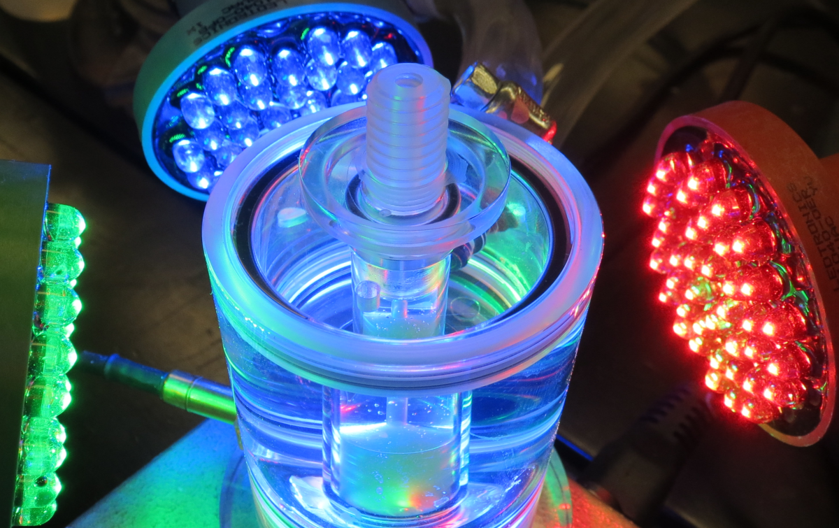
Illuminating Chloroplasts
From an anonymous lab group (Jennifer, Rachna and Kinsi)
Lab 07 Carbon Dioxide Coupling
Carbon Dioxide Coupling in Chloroplasts
In an intact chloroplast, production of oxygen should be related to the production of carbohydrate, a biochemical process that requires ATP and reducing equivalents (NADPH) produced in the light reaction of photosynthesis. So in this experiment, you will measure the complete biochemical machinery of the intact chloroplast by monitoring the effect of CO2 on oxygen evolution. The lab exercises on P/O Ratios and Carbon Dioxide Coupling are a test of your Experimental Hands. That is, how good you are at isolating high quality chloroplast suspensions that are as intact as possible. P/O Ratios require intact thylakoids, Carbon Dioxide Coupling requires an intact chloroplast, since the Calvin Cycle enzymes are located in the chloroplast stroma. It is your opportunity to replicate an historic experiment.
Additional stock solutions
- NaHCO3 100 mM (The NaHCO3 stock should be stored in an Ehrlenmeyer flask capped with a gas-tight rubber septum. Aliquots should be removed with a gas-tight syringe by penetrating the rubber septum with the needle. This is to avoid de-gassing of CO2 over time.)
- ADP 6 mM (keep on ice)
- NADP 6 mM (keep on ice)
Mix in a test tube:
- 1.0 ml of standard buffer (bubble with N2 to remove ambient levels of O2)
- 0.5 ml of chloroplasts (0.5 mg/ml stock in suspension medium)
- 0.1 ml of sodium phosphate
- 0.1 ml of MgCl2 6H2O
- 0.1 ml of NADP (the "real" final electron acceptor)
- 0.1 ml of ADP
- 0.1 ml of dH2O
Load the oxygen electrode cell with this mixture, insert the stopper, then let the cell come to an equilibrium temperature. Illuminate with a bright light until oxygen evolution has achieved a steady rate. Then inject 0.1 or 0.2 ml of NaHCO3 into the oxygen electrode cell. Observe the rate of oxygen evolution. Once the faster burst of oxygen evolution is complete and the rate has slowed to a steady rate, add an additional 0.1 or 0.2 ml of NaHCO3.
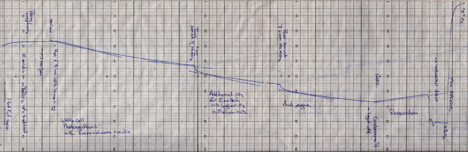
Carbon Dioxide Coupling in Algal Cells
If algal cells are available, the relation between extracellular [CO2] (added as NaHCO3) and O2 evolution will be examined in whole cells. They should be used at the same chlorophyll concentration as the isolated chloroplasts.
Here is an example. Note that oxygen evolution rates have not been calculated, but the oxygen calibration is shown at the end of the trace. Also, respiration by mitochondria is revealed during the dark treatment in these whole cells (something you shouldn't see in your chloroplast suspensions).
Calculations
Calculate and graph the relation between [NaHCO3] and O2 evolution.
INTERPRET
Carbon Dioxide Coupling in Chloroplasts
In historic research on chloroplasts, the 'Hill Reaction' was identified as light-driven oxygen production (in 1939, by Robert Hill). It's not uncommon for teaching labs (in high schools and first year university) to use a variant of the Hill reaction, in which an artificial electron acceptor is used in lieu of NADP. A common artificial electron receptor is DCIP (2,6 di-chlorophenol-indo-phenol). In its oxidized state, it is blue. When reduced, it is colorless:
DCIP(blue) + H2O -----------> DCIPH2 + 1/2 O2
The water is split in Photosystem II --producing oxygen-- and the electrons (and hydrogen ions) are donated to DCIP rather than NADP. So, oxygen evolution is measured indirectly by a colorimetric technique.
In the mid-1900's, scientists thought that carbon dioxide fixation into carbohydrate occurred elsewhere in the cell (not in the chloroplasts). This was because chloroplast isolation often damages the chloroplasts, and media used to measure oxygen production could inhibit carbon dioxide fixation. It wasn't until 1955 that scientists demonstrated that both oxygen production and carbon dioxide fixation occur in the chloroplast (Allen et al., 1955 Allen MB, Arnon DI, Capindale JB, Whatley FR, and Durham LJ (1955) Photosynthesis by isolated chloroplasts. III. Evidence for complete photosynthesis. Journal of the American Chemical Society 77:4149-4155.) using 14C labeling. It is now well established that the normal stoichiometry of oxygen evolution to carbon dioxide fixation O2:CO2 is 1:1 (Walker et al., 1968 Walker DA, Baldry CW and Cockburn W (1968) Photosynthesis by isolated chloroplasts, simultaneous measurement of carbon assimilation and oxygen evolution. Plant Physiology 43:1419-1422.). But note that a stoichiometry of 1:1 depends upon your skill in isolating intact chloroplasts! For algal cells, this is not a problem.
Chloroplast Molecular Biology
General Introduction
The chloroplast contains some, but not all, of the genetic information required to encode chloroplast proteins. The chloroplast DNA (cpDNA) is circular and about 40-500 um in circumference (sizes range from 80-280 kbp). Multiple copies are present in the chloroplast (about 300), often aggregated into multiple nucleoids, which are linked to the thylakoidal membrane. More than 120 genes encode for various proteins, in addition to the tRNAs and rRNAs required for protein synthesis within the chloroplast (which shares many attributes -gene organization and rRNA properties- with prokaryotes). Not all the proteins required for photosynthesis are encoded by the chloroplast genome. Many are encoded from the nuclear DNA, then imported into the chloroplast (see Lawlor Photosynthesis. 3d edition Chapter 10 for details). The inheritance of the chloroplast genome is complex: It may not be maternal, but instead bi-parental to varying degrees (due to plastid transfer from the pollen tube). Clearly, it is not Mendelian inheritance. The evolution of the chloroplast genome is only slowly beginning to be resolved, based on restriction mapping and sequencing of cpDNA from various phylogenetic lineages. In this two week lab exercise, we will (1) isolate the chloroplast DNA from separate species and (2) perform restriction mapping of the DNA.
| Parthenium Chloroplast Genome. This example of a chloroplast genome comes from Shashi Kumar, Frederick M Hahn, Colleen M McMahan, Katrina Cornish and Maureen C Whalen (2009) Comparative analysis of the complete sequence of the plastid genome of Parthenium argentatum and identification of DNA barcodes to differentiate Parthenium species and lines. BMC Plant Biology 2009, 9:131 [http://www.biomedcentral.com/1471-2229/9/131]. Parthenium is a latex-producing industrial crop plant. |  |
Chloroplast Genome DNA Isolation
The isolation of the chloroplast genome relies upon the isolation of intact chloroplasts with minimal cross-contamination by the nuclear genomic DNA. Often, this involves the initial preparation of intact chloroplasts which are then treated with DNase to removed nuclear DNA contaminants. The problem that arises is that multiple purifications and enzymatic treatments result in very low yields of the chloroplast genome. Thus, in the protocols we will use, DNase treatment is not performed.
Lab 08 Isolation of Chloroplast DNA
General Objective
To isolate the chloroplast genome from photosynthetic organisms. The isolated DNA will be used for restriction mapping.Flow Sheet: Isolation of Chloroplast DNA Special thanks to Melissa Begin, Debbie Freele and Maria Mazzurco for developing and testing the flow sheet.
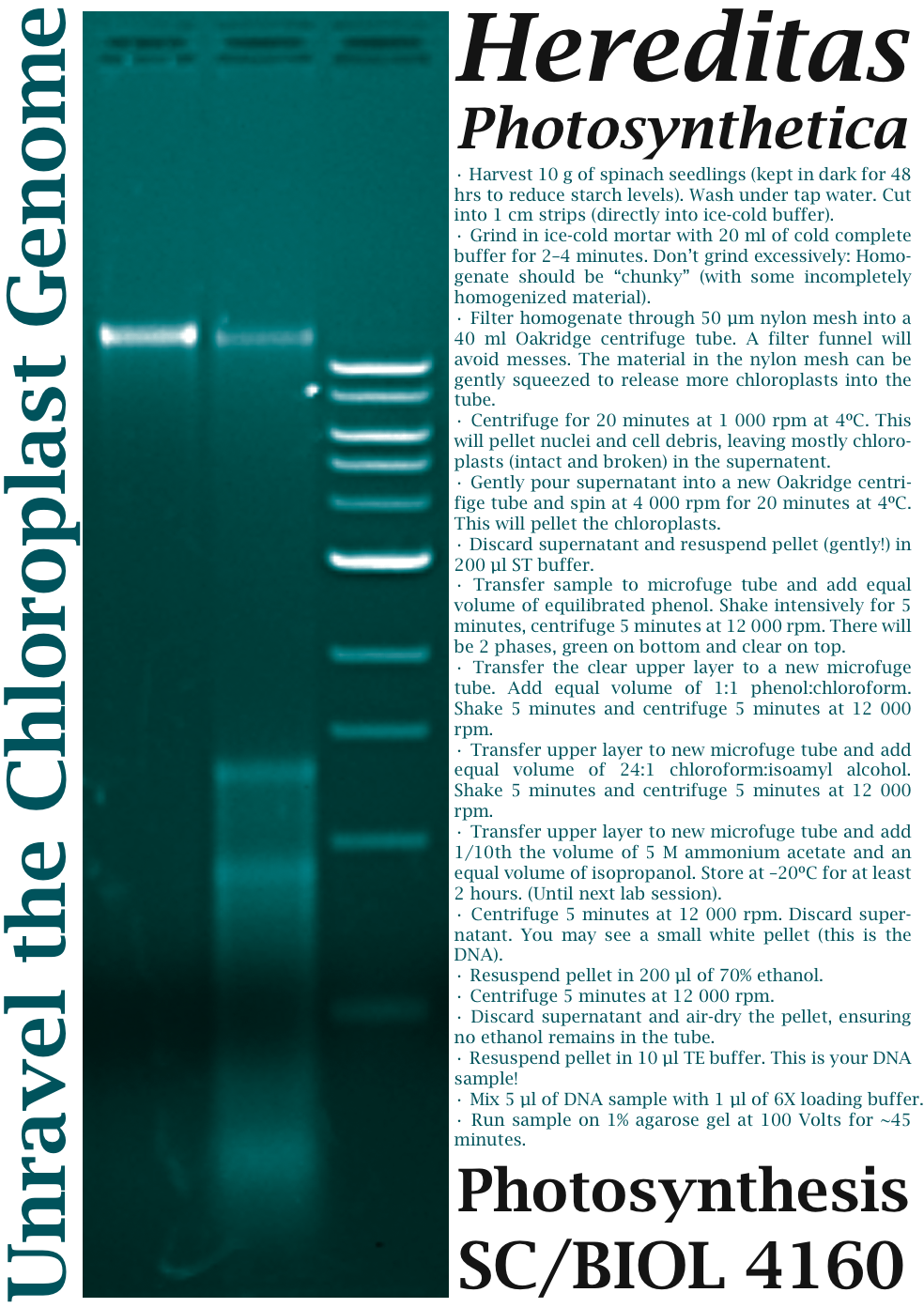
- Harvest 10 g of spinach seedlings (kept in dark for 48 hrs to reduce starch levels). Wash under tap water. Cut into 1 cm strips (directly into ice-cold buffer).
- Grind in ice-cold mortar with 20 ml of cold complete buffer (STE) for 2-4 minutes. Don't grind excessively: Homogenate should be “chunky” (with some incompletely homogenized material).
- Filter homogenate through 50 um nylon mesh into a 40 ml Oakridge centrifuge tube. A filter funnel will avoid messes. The material in the nylon mesh can be gently squeezed to release more chloroplasts into the tube.
- Centrifuge for 20 minutes at 1 000 rpm at 4ºC. This will pellet nuclei and cell debris, leaving mostly chloroplasts (intact and broken) in the supernatent.
- Gently pour supernatant into a new Oakridge centrifige tube and spin at 4 000 rpm for 20 minutes at 4ºC. This will pellet the chloroplasts.
- Discard supernatant and resuspend pellet (gently!) in 200 ul ST buffer.
- Transfer sample to microfuge tube and add equal volume of equilibrated phenol. Shake intensively for 5 minutes, centrifuge 5 minutes at 12 000 rpm. There will be 2 phases, green on bottom and clear on top.
- Transfer the clear upper layer to a new microfuge tube. Add equal volume of 1:1 phenol:chloroform. Shake 5 minutes and centrifuge 5 minutes at 12 000 rpm.
- Transfer upper layer to new microfuge tube and add equal volume of 24:1 chloroform:isoamyl alcohol. Shake 5 minutes and centrifuge 5 minutes at 12 000 rpm.
- Transfer upper layer to new microfuge tube and add 1/10th the volume of 5 M ammonium acetate and an equal volume of isopropanol. Store at -20ºC for at least 2 hours. (Until next lab session).
- Centrifuge 5 minutes at 12 000 rpm. Discard supernatant. You may see a small white pellet (this is the DNA) or not (sometimes, the pellet is clear and hard to see even though the DNA is there!).
- Resuspend pellet in 200 ul of 70% ethanol. Centrifuge 5 minutes at 12 000 rpm.
- Discard supernatant and air-dry the pellet, ensuring no ethanol remains in the tube.
- Resuspend pellet in 10 ul TE buffer. This is your DNA sample!
- This is what you will use for your restriction enzyme digests.
- Mix 5 ul of DNA sample with 1 ul of 6X loading buffer.
- Run sample on 1% agarose gel at 100 Volts for ~45 minutes.
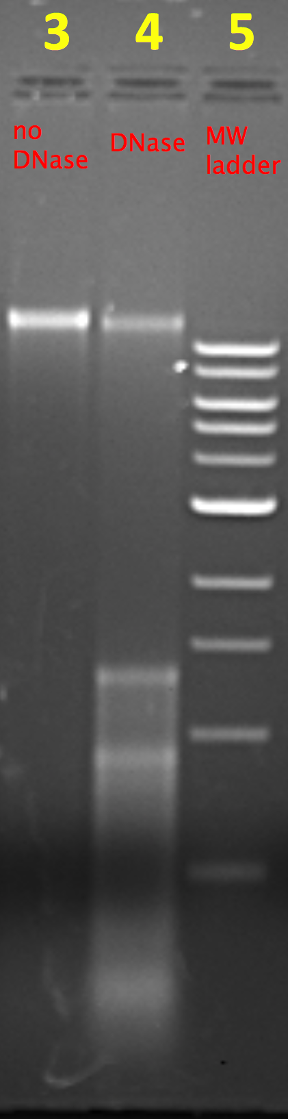
Gel Electrophoresis of Chloroplast Genome
Here is an example of a gel (by students in the course!). The first lane (3) shows a band with a molecular weight higher than any of the bands in the DNA molecular weight ladder (5). This is the circular chloroplast "chromosome". The actual size of the chloroplast circular DNA cannot be calculated because it is supercoiled (coiled together into a 'knot', making its size smaller than the relaxed circular DNA, causing it to run faster in the gel). The actual size of the chloroplast 'chromosome' ranges from 80-280 kb, depending on species. The second lane (4) shows additional DNA fragments created as a consequence of DNase treatment. The third lane (5) is the molecular ladder: In descending order, 10 / 8 / 6 / 5 / 4 / 3 / 2 / 1.5 / 1 / 0.5 kb.Solutions
STE
|
ST
|
TE
|
Lab 09 Chloroplast Genome Mapping
General Objective
To obtain a restriction map of the chloroplast genome.The sequence of the spinach chloroplast genome is available (Christian Schmitz-Linneweber, Rainer M. Maier, Jean-Pierre Alcaraz, Annick Cottet, Reinhold G. Herrmann,and Regis Mache (2001) The plastid chromosome of spinach (Spinacia oleracea): complete nucleotide sequence and gene organization. Plant Molecular Biology 45:307-315.). The sequence is available as a text file here [at http://www.bch.umontreal.ca/ogmp/projects/other/genbank/AJ400848.txt] (http://megasun.bch.umontreal.ca/ogmp/projects/other/cp_list.html) or at NCBI [http://www.ncbi.nlm.nih.gov/nuccore/AJ400848]. In your lab exercise, you will be provided with some choices of restriction enzymes, and the protocols for DNA digestion.
Here is an example of restriction sites for the spinach chloroplast genome
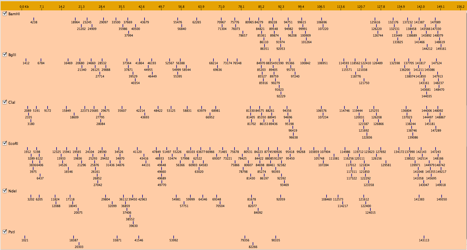
Restriction Enzyme Digest Protocol
How to set up a Digest
- Add the following components to an eppendorf tube adding the restriction enzyme last
- 3 uL DNA
- 1 uL restriction enzyme
- 1 uL 10X Buffer 3
- 1 uL 10X BSA
- 3 uL ddH2O
- Quickly mix contents of the tube and place eppendorf tube in a 37oC water bath for 45 minutes
- Remove tube from the water bath and add 2 uL of 6X loading buffer
- Shake tube and quick spin to collect contents of the tube.
- Load all 12 uL of the digest onto the 0.8% agarose gel.
- Let run at 100 Volts for approximately 45 minutes.
- Look at gel under UV light.
- Add 3 uL DNA to a clean eppendorf tube.
- Add 7 uL of ddH2O and 2 uL of 6X loading buffer.
- Load all 12 uL onto the 0.8% gel.
- Replace only the Pst1 with Bgl II.
- Follow all the same instructions.
- Add
- 3 uL DNA
- 1 uL Pst I
- 1 uL Bgl II
- 1 uL 10X Buffer 3
- 1 uL 10X BSA
- 3 uL ddH2O
- Follow all the same instructions.
Chloroplast Genomic DNA Digest
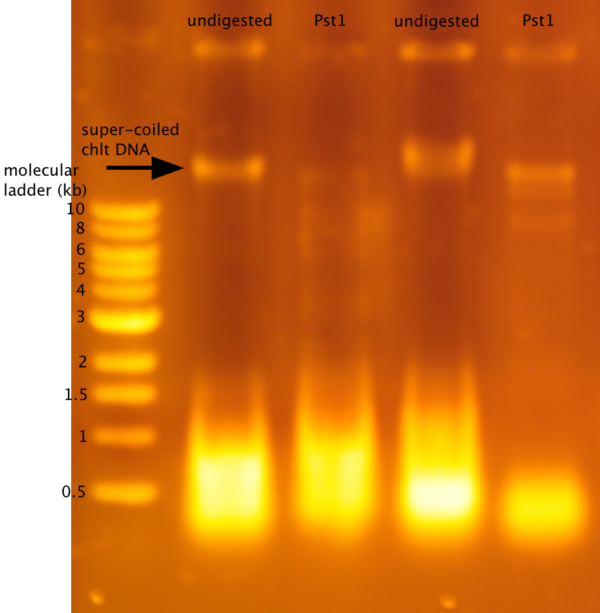
Lab 10 Presentations: Pathways of Carbon Dioxide Fixation
General Introduction
| Figure 1. Carbon Pathways |
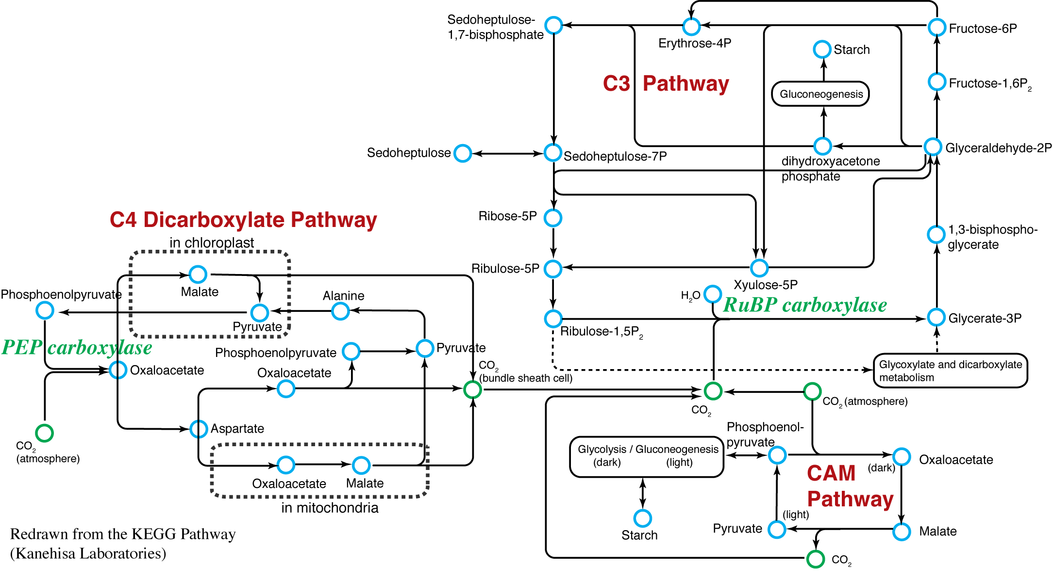 |