1.5 A Rigorous Formulation of Agents' Decision
Having explained the relation between indifference curves and utility functions and the meaning of a unity function we are now in a position to pose the problem solved by the agents. Assume that the price of good 1 is ![]() and that of good 2 is
and that of good 2 is ![]() and that the agent has a budget of
and that the agent has a budget of ![]() and a utility function
and a utility function ![]() . The reader may have already guessed that the agent needs to solve a maximization problem which is formulated as below:
. The reader may have already guessed that the agent needs to solve a maximization problem which is formulated as below:
![]()
s.t. ![]()
![]()
![]()
Since ![]() is a monotone increasing function, the inequality
is a monotone increasing function, the inequality ![]() can be replaced with an equality
can be replaced with an equality ![]() . Thus, one way of solving this problem is by substituting
. Thus, one way of solving this problem is by substituting ![]() in terms of
in terms of ![]() and solving an optimization problem with only the non-negativity constraints
and solving an optimization problem with only the non-negativity constraints ![]()
![]() .
.
We will, however, utilize this opportunity to review the optimality conditions as they play a central role in the portfolio choice problem. Furthermore, we will explain or provide a heuristic proof for the optimality conditions. This proof highlights a relation (duality) between two systems of inequalities that is used later in the Arbitrage Pricing Theory (APT).
In order to state the optimality conditions in a generic way we should decide about a canonical form of an optimization problem. We will define a canonical form as a minimization problem with constraints of the type ![]() . That is, a problem of the form
. That is, a problem of the form
![]()
s.t. ![]() ,
, ![]()
Where ![]() is a vector in
is a vector in ![]() and
and ![]() and
and ![]() ,
, ![]() are functions from
are functions from ![]() to
to ![]() and
and ![]() ,
, ![]() .
.
It is easy to see that there is no loss of generality assuming such a canonical form of an optimization problem. The solution of a maximization problem is the same for a minimization problem in which the negative of the objective function ![]() is minimized. Inequality constraints could be reversed by multiplying the inequality by
is minimized. Inequality constraints could be reversed by multiplying the inequality by ![]() and an equality can be written as a pair of two inequalities. After we develop the optimality condition for the above problem we will apply it to our maximization of utility problem.
and an equality can be written as a pair of two inequalities. After we develop the optimality condition for the above problem we will apply it to our maximization of utility problem.
Let us first start with the intuition behind the optimality conditions. If ![]() is a minimum point of
is a minimum point of ![]() , subject to the constraint stipulated above, it must be that there is no feasible direction
, subject to the constraint stipulated above, it must be that there is no feasible direction ![]()
![]() “along which one can move away” from
“along which one can move away” from ![]() and reach a point where the value of
and reach a point where the value of ![]() is smaller than the value of
is smaller than the value of ![]() at
at ![]() . Being a feasible point,
. Being a feasible point, ![]() satisfies the constraint, that is
satisfies the constraint, that is ![]() ,
, ![]() . The direction
. The direction ![]() is feasible if there exists an
is feasible if there exists an ![]() ", mathvariant = "normal", fence = "false", separator = "false", stretchy..." align="center" border="0"> such that
", mathvariant = "normal", fence = "false", separator = "false", stretchy..." align="center" border="0"> such that ![]() ,
, ![]() . Moving away from
. Moving away from ![]() along the direction
along the direction ![]() , will lead to a point
, will lead to a point ![]() for some positive
for some positive ![]() .
.
![]()
![]() , for a given
, for a given ![]() and
and ![]() in
in ![]() .
.
![]() thus equals
thus equals ![]() , and if
, and if ![]() is negative it means that moving along the direction
is negative it means that moving along the direction ![]() ,
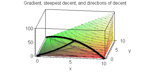
, ![]() decreases. Footnote 6 A visualization of direction of decent relative to the gradient and the value of the function along these directions is offered below for the utility function of the former section. The graph below demonstrates the direction
decreases. Footnote 6 A visualization of direction of decent relative to the gradient and the value of the function along these directions is offered below for the utility function of the former section. The graph below demonstrates the direction ![]() for
for ![]() at a point (5,5).
at a point (5,5).
The directions of the negative of the gradient is drawn as a black line in the ![]() axis that points to the origion, with two other directions that are perpendicular to it. All the direction between the two prepndcualr directions are directions of decent. The movement along these directions is also drawn on the graph of the function so one can realize that these are indeed directions of decent.
axis that points to the origion, with two other directions that are perpendicular to it. All the direction between the two prepndcualr directions are directions of decent. The movement along these directions is also drawn on the graph of the function so one can realize that these are indeed directions of decent.
| > | NGFradNfun:=plot3d([[5-x,5-x,(5-x)*(5-x)],[5-x,5-x,0],[5-x,5+x,(5-x)*(5+x)],[5+x,5-x,(5+x)*(5-x)],[5-x,5+x,0],[5+x,5-x,0]],x=0..5,y=0..5,axes=box,thickness=4): |
| > |
| > | Util:=plot3d(x*y,x=0..10,y=0..10,axes=box,style=patchcontour,contours = 20,filled=true,orientation=[-82,56],title="Gradient, steepest decent, and directions of decent ",transparency=.2): |
| > |
| > | plots[display](Util,NGFradNfun); |
 |
| > |
| > |
Similarly if ![]() is a point on the boundary of the feasible set, i.e., it satisfies one of the constraints say
is a point on the boundary of the feasible set, i.e., it satisfies one of the constraints say ![]() as equality rather than inequality, and if the function
as equality rather than inequality, and if the function ![]() is such that
is such that ![]()
![]() is not a feasible direction. This is because as we move along
is not a feasible direction. This is because as we move along ![]() ,
, ![]() increases and since at
increases and since at ![]() ,
, ![]() there exists an
there exists an ![]() ", mathvariant = "normal", fence = "false", separator = "false", stretchy = "false", symmetric =..." align="center" border="0">such that
", mathvariant = "normal", fence = "false", separator = "false", stretchy = "false", symmetric =..." align="center" border="0">such that ![]() violates the constraint since
violates the constraint since ![]() for every ε in
for every ε in ![]()
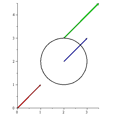
This is illustrated below where the vector ![]() is the red line. Moving along
is the red line. Moving along ![]() with
with ![]() .5 from the point (2,3) is demonstrated by the green line which leads to the point
.5 from the point (2,3) is demonstrated by the green line which leads to the point ![]() . Moving along
. Moving along ![]() from the point (2,2) with
from the point (2,2) with ![]() is demonstrated by the blue line which ends at
is demonstrated by the blue line which ends at ![]() . The feasible set is demonstrated by the black circle and one can visualize that the direction
. The feasible set is demonstrated by the black circle and one can visualize that the direction ![]() from the point (2,2) is a feasible direction as it is possible to move along it and still stay within the feasible set. On the other hand the direction
from the point (2,2) is a feasible direction as it is possible to move along it and still stay within the feasible set. On the other hand the direction ![]() is not a feasible direction from the point (2,3) since moving along it, even with a very small positive
is not a feasible direction from the point (2,3) since moving along it, even with a very small positive![]() , will result in a point outside the feasible set. The feasible set in this illustration is given by the function
, will result in a point outside the feasible set. The feasible set in this illustration is given by the function
![]() .
.
| > | V11:=plots[arrow]([<1,1>], width=[0.02, relative], head_length=[0.04, relative], color=red): |
| > | V1122:=plots[arrow](<2,2>,<1,1>, width=[0.02, relative], head_length=[0.04, relative], color=blue): |
| > | V1123:=plots[arrow](<2,3>,<1.5,1.5>, width=[0.02, relative], head_length=[0.04, relative], color=green): |
| > | FeasC:=plot([[2+cos(t),2+sin(t), t=0..2*Pi]], color=[black],thickness=2,scaling=constrained): |
| > | plots[display](V11,V1122,V1123,FeasC); |
 |
| > |
| > |
The derivative of![]() with respect to
with respect to ![]() is given by
is given by ![]() where ▽ denotes the gradient of
where ▽ denotes the gradient of ![]() (the vector of partial derivatives) and
(the vector of partial derivatives) and ![]() denotes the transpose of
denotes the transpose of ![]() (a row vector). At the point
(a row vector). At the point ![]() ,
, ![]() is positive if
is positive if ![]() At the point (2,3) we can calculate
At the point (2,3) we can calculate ![]() as below
as below
| > | Student:-MultivariateCalculus:-Gradient((x-2)^2+(y-2)^2,[x,y]=[2,3]); |
| > |
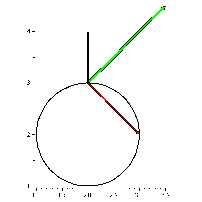
In the graph below the gradient of ![]() at the point (2,3) is illustrated by the blue line, the direction
at the point (2,3) is illustrated by the blue line, the direction ![]() from the point
from the point ![]() by the green line, and the direction
by the green line, and the direction ![]() from the point
from the point ![]() by the red line.
by the red line.
| > | V0123:=plots[arrow](<2,3>,<0,1>, width=[0.02, relative], head_length=[0.04, relative], color=blue): |
| > | V1Neg123:=plots[arrow](<2,3>,<1,-1>, width=[0.02, relative], head_length=[0.04, relative], color=red): |
| > | plots[display](V1123,V0123,V1Neg123,FeasC); |
 |
| > |
You may recall that if ![]() than the angle between the vector
than the angle between the vector ![]() and
and ![]() is acute, while if the angle between the vector
is acute, while if the angle between the vector ![]() and
and ![]() is obtuse
is obtuse ![]() . In the case illustrated above by the green line
. In the case illustrated above by the green line ![]() since
since ![]() and hence the angle between the vector
and hence the angle between the vector ![]() and
and ![]() is acute and the green line is not a feasible direction.
is acute and the green line is not a feasible direction. ![]()
On the other hand the direction ![]() is a feasible direction from the point
is a feasible direction from the point ![]() . It is represented by the red line which points inside the circle. On the circle the value of
. It is represented by the red line which points inside the circle. On the circle the value of ![]() is 1 and inside the circle it is less than 1. Hence moving along this direction does not violate the constraint that requires that
is 1 and inside the circle it is less than 1. Hence moving along this direction does not violate the constraint that requires that ![]() Feasible directions are therefore those that generate an obtuse angle with the gradients of the binding constraints. A feasible direction
Feasible directions are therefore those that generate an obtuse angle with the gradients of the binding constraints. A feasible direction ![]() at a point
at a point ![]() , is characterized by the fact that for each binding constraint
, is characterized by the fact that for each binding constraint ![]() at
at ![]() , i.e., for each
, i.e., for each ![]() for which
for which ![]() , the product of
, the product of ![]() and the gradient of
and the gradient of ![]() is negative, that is
is negative, that is ![]()
If the point is a minimum point, it must be that there exists no feasible direction along which the objective function decreases. Footnote 7 Since if one existed there would be a feasible point say ![]() =
=![]() for some γ>0 such that
for some γ>0 such that ![]() , but that means that
, but that means that ![]() could not be the minimum point. Thus, if
could not be the minimum point. Thus, if ![]() is a minimum point it must be that
is a minimum point it must be that
![]() for every
for every ![]() such that
such that ![]() then
then ![]() ,
,
i.e., the function ![]() increases along each feasible direction
increases along each feasible direction ![]() from
from ![]() .
.
This condition can also be stated as:
Every ![]() such that
such that ![]() for
for ![]() such that
such that ![]() , must satisfy
, must satisfy ![]() .
.
Put into words, every feasible direction from point ![]() , must be a direction along which
, must be a direction along which ![]() does not decrease. This condition can also be geometrically visualized.
does not decrease. This condition can also be geometrically visualized.
Assume that there are two binding constraints at a point ![]() , hence we have vectors representing the gradient of
, hence we have vectors representing the gradient of ![]() , and
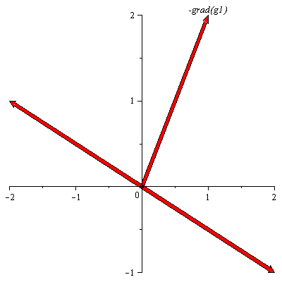
, and ![]() . A feasible direction must make an acute angle with each of these vectors. We start by plotting a vector representing
. A feasible direction must make an acute angle with each of these vectors. We start by plotting a vector representing ![]() and the vectors that are making an acute angle with it. Assume that
and the vectors that are making an acute angle with it. Assume that ![]() is the vector
is the vector ![]() . Two vectors that make a right angle with it are given by
. Two vectors that make a right angle with it are given by ![]() and
and ![]() , hence vectors that are making an acute angle with
, hence vectors that are making an acute angle with ![]() are between these two vectors. (Note the vectors that make a right angle with
are between these two vectors. (Note the vectors that make a right angle with ![]() must have a product of zero with it, e.g.,
must have a product of zero with it, e.g., ![]() . This is illustrated below:
. This is illustrated below:
| > | Lg1:=plots[textplot]([1,2,`-grad(g1)`],align=ABOVE): |
| > | Neggradg1:=plots[arrow]({<1,2>,<-2,1>,<2,-1>}, width=[0.02, relative], head_length=[0.04, relative], color=red): |
| > | plots[display](Lg1,Neggradg1); |
 |
| > |
The vectors that are making an acute angle with![]() are those that are between the two vectors making a right angle with it. These are the vectors with an end point above the red line (that passes via the origin).
are those that are between the two vectors making a right angle with it. These are the vectors with an end point above the red line (that passes via the origin).
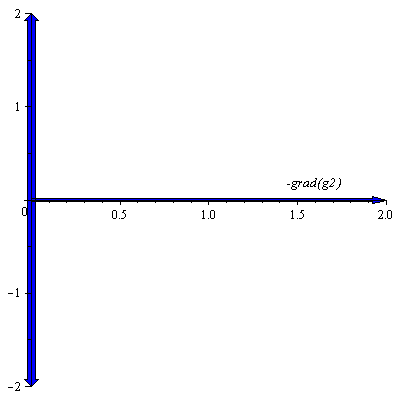
Assume that ![]() and let us now graph
and let us now graph ![]() and all the vectors making an acute angle with it. This can still be displayed in the figure below.
and all the vectors making an acute angle with it. This can still be displayed in the figure below.
| > | Neggradg2:=plots[arrow]({<2,0>,<0,-2>,<0,2>}, width=[0.02, relative], head_length=[0.04, relative],color=blue): |
| > | Lg2:=plots[textplot]([1.6,0.1,`-grad(g2)`],align=ABOVE): |
| > | plots[display](Lg2,Neggradg2); |
 |
| > |
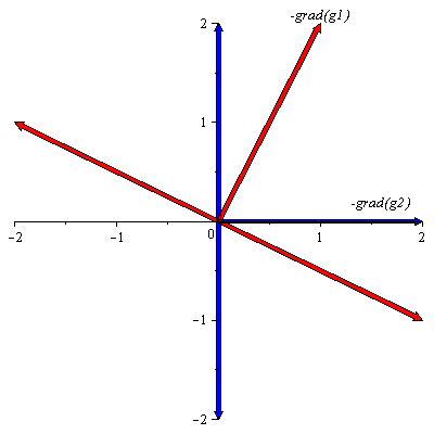
Let us now visualize the vectors that are making acute angles with both![]() and
and![]() This will be the intersection of the two sets of vectors described in the above two graphs. That is the vectors with an end point above the red line that passes via the origin, and to the left of the blue line that passes through the origin.
This will be the intersection of the two sets of vectors described in the above two graphs. That is the vectors with an end point above the red line that passes via the origin, and to the left of the blue line that passes through the origin.
| > | plots[display](Lg1,Neggradg1,Lg2,Neggradg2); |
 |
| > |
Recall that if ![]() is a minimum point, the angle between each feasible
is a minimum point, the angle between each feasible![]() and
and![]() must also be acute, that is
must also be acute, that is ![]() for every
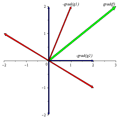
for every ![]() which is a feasible direction. Observing the set of feasible directions in the graph above, the reader should realize that for
which is a feasible direction. Observing the set of feasible directions in the graph above, the reader should realize that for![]() to make an acute angle with each feasible
to make an acute angle with each feasible ![]() ,
, ![]() must be between
must be between ![]() and
and ![]() An example of a vector that satisfies this condition is illustrated below. It is labeled as grad(f) and it is the green vector in the graph below:
An example of a vector that satisfies this condition is illustrated below. It is labeled as grad(f) and it is the green vector in the graph below:
| > | gradf:=plots[arrow](<3,2>, width=[0.02, relative], head_length=[0.04, relative],color=green): |
| > | Lf:=plots[textplot]([2.7,2,`grad(f)`],align=ABOVE): |
| > | plots[display](Lg1,Neggradg1,Lg2,Neggradg2,gradf,Lf); |
 |
| > |
However algebraically for ![]() to be between
to be between ![]() and
and ![]() it means that
it means that ![]() is a positive linear combination of
is a positive linear combination of ![]() and
and ![]() i.e.,
i.e., ![]() =
=![]()
![]() for some positive
for some positive ![]() and
and ![]() In general therefore, this condition is satisfied if
In general therefore, this condition is satisfied if ![]() is a positive linear combination of
is a positive linear combination of ![]() , for
, for ![]() such that
such that ![]() . That is
. That is ![]() where the summation is over
where the summation is over ![]() such that
such that ![]() and the
and the ![]() are all nonnegative. Footnote 8
are all nonnegative. Footnote 8
We are now ready to stipulate the optimality conditions for the canonical minimization problem. It is common to stipulate the optimality conditions in terms of a function called Lagrangian, associated with the canonical optimization problem. The Lagrangian of our canonical minimization problem is defined to be a function of ![]() , a vector in
, a vector in ![]() (
(![]() is the number of constraints) and
is the number of constraints) and ![]() .
.
![]()
The optimality conditions are stated in terms of the partial derivative of the Lagrangian ![]() below:
below:
![]() i=1,...,n
i=1,...,n
![]()
![]() j=1,...,m
j=1,...,m
![]() j=1,...,m
j=1,...,m
The reader is asked to verify that the first condition above states that ![]() , the third condition ensures that if the
, the third condition ensures that if the ![]() constraint is not binding
constraint is not binding ![]() =0 and hence the sum in
=0 and hence the sum in ![]() is only over the binding constraints. Finally the second constraint simply guarantees that
is only over the binding constraints. Finally the second constraint simply guarantees that ![]() is a feasible point and satisfies the constraints.
is a feasible point and satisfies the constraints.
In our utility maximization problem, ![]() is
is ![]() , (
, (![]() and
and ![]() are
are ![]() and
and ![]() ), the non-negativity constraints on
), the non-negativity constraints on ![]() and
and ![]() can be written in terms of the
can be written in terms of the ![]() , and we also have one inequality constraint that can be written as an equality constraint
, and we also have one inequality constraint that can be written as an equality constraint ![]() because of the monotonic of
because of the monotonic of ![]() . The equality constraint can be written as two inequality constraints.
. The equality constraint can be written as two inequality constraints.
The reader is asked to show that this will alter the optimal conditions only by allowing the ![]() associated with this constraint to be positive or negative instead of the nonnegative constraint that is imposed on λ that is associated with an inequality constraint of the type less than or equal. Our problem is a maximization problem. We can transform the maximization of
associated with this constraint to be positive or negative instead of the nonnegative constraint that is imposed on λ that is associated with an inequality constraint of the type less than or equal. Our problem is a maximization problem. We can transform the maximization of ![]() to a minimization of
to a minimization of ![]() . Therefore we have
. Therefore we have
![]()
s.t. ![]()
![]()
Writing the Lagrangian of this problem and the optimality conditions where, ![]() and
and ![]() are associated with
are associated with
the non-negativity constraints on ![]() and
and ![]() respectively, yields:
respectively, yields:
If we assume that the non-negativity constraints on ![]() and
and ![]() are not binding, that is that the optimal solution is an interior point of the positive orthant we can try to satisfy the equations:
are not binding, that is that the optimal solution is an interior point of the positive orthant we can try to satisfy the equations:
![]()
![]()
which implies that

or that

Note that ![]() is the slope of the budget line and
is the slope of the budget line and![]()
 is the slope of the indifference curve. Since
 ![]() we have the second equation:
we have the second equation:
![]()
Solving these two equations will thus produce the same solution as produced by the graphical procedure.
We conclude this chapter with an example. Consider the optimization problem
![]()
s.t. ![]()
![]()
![]()
Where ![]() ,
, ![]() ,
, ![]() and
and ![]()
![]() . The KT optimality conditions of this problem are:
. The KT optimality conditions of this problem are:
![]()
![]()
![]()
![]()
![]()
![]()
This system of equalities and inequalities can be solved by Maple as demonstrated below.
| > | solve({c1+c2/(1.14)=80,-diff(c2+1.07*c1,c1)+lambda+eta||1=0,\
-diff(c2+1.07*c1,c2)+lambda*(1/1.14)+eta||2=0,\ c1>=0,c2>=0,eta||1<=0,eta||2<=0,eta||1*c1=0,eta||2*c2=0},\ {c1,c2,lambda,eta||1,eta||2}); |
| > |
One of the exercises at the end of the chapter asks the reader to solve this problem using the graphing approach (which can also be done using our procedure BudnIndif(c1+c2/1.14, c2+1.07c2)) and to explain and compare the results of the graphical approach with that of the formal approach using KT conditions.