6. RESULTS AND DISCUSSION

6.1 Plan for Analysis

This chapter presents and discusses the results of the three experiments. For each, the plan for analysis is as follows. First, adjustments to the data are introduced to minimize learning effects and to eliminate outliers. Then, summary measures and tests for main effects and interactions are presented on movement time, error rate, etc., across levels of experimental factors. Finally, correlation and regression analyses are presented to test and compare the models under investigation. The data analysis was performed on a VAX minicomputer using SPSSx release 3.1.

There are sufficient model variations and sufficient "views" of the data that the potential exists to overwhelm the reader with statistics. For example, in the first experiment an important statistic is Fitts' index of performance (IP ). Figure 17 illustrates four dimensions of analysis along which IP may be obtained: (a) using unadjusted or adjusted data; (b) using the direct method (Equation 2) or linear regression; (c) using the Fitts, Welford, or Shannon formulation; or (d) using the specified or effective target width. Since all combinations are possible, there are 2 × 2 × 3 × 2 = 24 possible outcomes for each of the six device-task conditions. It is digressive to tabulate all 144 IPs and proceed to explore the differences. Furthermore, for each cell in Figure 17 numerous other statistics are of potential interest, such as the standard deviation or, under linear regression, the standard error, correlation, or intercept.

Figure 17. Possible ways to obtain Fitts' index of performance

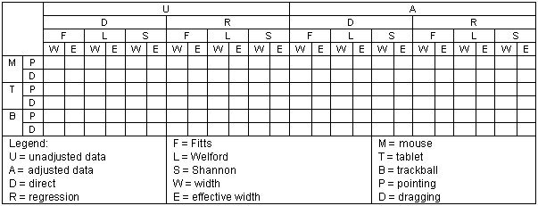
As results are presented, it will be clearly stated what "dimension of analysis" is in effect. Although countless other measures could be presented showing different views of the data, their absence is aimed at maintaining purpose in the discussion.

6.2 Experiment 1

6.2.1 Adjustment of Data

A Newman-Keuls test was used to identify learning effects over the five session means. The test was applied at the p < .05 level for each device-task condition and for three dependent variables: movement time (MT ), error rate, and the index of performance (IP ). IP was calculated using Shannon formulation and using the effective target width (using the SD method). The effective target width is preferred because it allows IP to reflect the speed and accuracy of movements.

Three device-task conditions showed no significant difference in movement times over the five sessions and three showed that session MTs were significantly longer during session one than during groupings of other sessions. For error rate, there was no significant difference between the session means for any device-task condition. For IP, there was no significant difference under four conditions and significant differences under two conditions with session one showing a significantly lower rate of information processing than sessions four and five. It was decided that learning effects would be largely reduced by removing data for the first session for all device-task conditions.

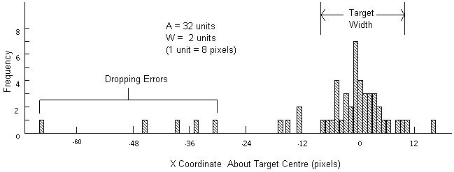
On the remaining data, a criterion was introduced to eliminate outliers. Subjects were observed to occasionally "drop" the object during the dragging task, not through normal motor variability, but because of difficulty in sustaining State 2 motion. (This was particularly evident with the trackball.) Thus "dropping errors" were distinguished from errors due to random neuromotor variability. Examining the distribution of "hits" (the x coordinates) confirmed this source of error. Figure 18 shows one subject's spatial distribution of responses around the target for 50 trackball-dragging trials with A = 32 and W = 2. The data reveal deviate responses at very short movement distances distinct from the normal variability expected.

Figure 18. Sample distributions of responses

Because dropping errors are considered a distinct behaviour, the data were further adjusted by eliminating trials with an x coordinate more than three standard deviations from the mean. Means and standard deviations were calculated for each subject and for each device-task-amplitude-width condition.

Trials immediately following deviate responses were also eliminated. The literature on response times for repetitive, self-paced, serial tasks suggests that deviate trials are disruptive events and can cause unusually long response times on the following trial (Rabbitt, 1968; Worringham, 1989). Of the 46,080 trials for sessions two through five, 822 or 1.8% were dropped. Total trials removed for the mouse, tablet, and trackball respectively were 83, 91, and 83 during pointing, and 133, 171, and 261 during dragging.

Except where indicated, subsequent analyses used adjusted data.

6.2.2 Distribution Characteristics

The distribution in Figure 18 is atypical. It is highly skewed (sk = −2.40) and leptokurtic (ku = 6.76). The adjusted data were examined in an effort to determine the overall distribution characteristics of the spatial coordinates. Since the method for calculating the effective target width assumes a normal distribution (see Figure 4), tests for skewness, kurtosis, and normality should precede the adjustment.

Skewness and kurtosis were calculated for each subject and for each device-task-amplitude-width condition (1152 samples, n ≈ 40 points/sample). The mean skewness was −0.40 (SD = 1.59) and the mean kurtosis was 3.73 (SD = 7.94). The relatively large standard deviations in these statistics resulted from a small number of samples still containing a few extreme deviate responses (even after adjustment). The 10 and 90 percentiles respectively were −2.72 and 0.83 for skewness and −0.50 and 11.87 for kurtosis. The large kurtosis is disturbing; however, as Glass and Hopkins (1984, p. 70) note, skewness in itself tends to yield a leptokurtic distribution because of the disproportionate number of points a significant distance from the mean. Regardless, and as also noted, kurtosis is generally of much less importance than skewness in characterizing distributions.

A chi-square goodness-of-fit test was used to compare the observed distributions against a normal distribution. To maintain a reasonably large n for each cell, subject responses were pooled and the test was applied to each device-task-amplitude-width condition (96 samples, n ≈ 480 points/sample). The x coordinates of selection were grouped into eight cells spanning the width of the target. Two additional cells were assigned for selections on either side of the target. The eight centre cells each contained counts for selections on a single pixel for W = 1 unit, selections on two adjacent pixels for W = 2 units, and so on. (Recall that 1 unit = 8 pixels.) The expected frequencies were generated using a cumulative frequency distribution function for the normal curve. Since m and s were estimated from the sample mean and standard deviation, two additional degrees of freedom were lost. Tests for the null hypothesis — that the selection coordinates formed a normal distribution — proceeded using the chi-square statistic with df = 7.

Of the 96 samples tested, the null hypothesis was tenable 39 times (p > .05). Of these, only 3 samples were for the dragging task while 36 were for the pointing task (12 for the mouse, 9 for the tablet, & 15 for the trackball). No trend was evident across amplitude-width conditions. It is apparent that the dragging task still contained deviate responses even after the criteria for eliminating outliers were applied. However, the assumption of normality remains plausible for the pointing task.

The 96 means for selection coordinates revealed the extent to which subjects "went the distance" in realizing the tasks. Although there was a slight negative tendency in the means — implying the mean distance travelled was less than A, no mean deviated from zero by more than two pixels. Therefore, the earlier suggestion that model building may be improved using the "effective target amplitude" (see p. 27) was not pursued further.

6.2.3 Summary Tables

A goal of this experiment was to compare the performance of several device-task combinations using Fitts' information processing model. Since the experimental design specifically mimicked Fitts' original tapping experiments, tables similar to Table 1 (see p. 14) form the basis for subsequent analyses. Table 9 is an example showing for the mouse-pointing condition the means for movement time, error rate, and the index of performance across levels of A and W. Similar tables for all device-task conditions are found in Appendix B (see p. 155). As in Table 1, Table 9 includes both the specified target width (W ) and the effective target width. However, unlike Fitts' experiments in which only discrete errors were recorded, the present experiment recorded the coordinates of target selection; thus the effective target width could be equated using both the discrete error method, W_e(DE ), and the standard deviation method, W_e(SD ). Although the latter method is considered superior (see p. 21), both are shown in Table 9 to maintain consistency with Table 1 and to facilitate comparisons. For the same reasons, ID and IP were derived using Fitts' formulation (although they can be re-calculated using the Welford or Shannon formulation with the data provided).

Table 9
Summary Data for the Mouse-Pointing Condition

A a	W a	W e(SD) a	W e(DE) a	ID (bits) b	MT (ms)	Errors (%)	IP (bits/s)	Trials
8	8	4.232	5.370	1	221	.21	4.72	474
8	4	3.055	3.388	2	331	1.47	6.26	472
16	8	5.691	6.266	2	303	.83	6.85	477
8	2	1.738	1.817	3	488	2.29	6.35	478
16	4	3.208	3.309	3	450	1.25	6.84	476
32	8	6.235	6.462	3	445	1.05	6.83	476
8	1	1.004	1.110	4	663	6.27	6.15	474
16	2	1.839	1.871	4	620	2.72	6.54	478
32	4	3.134	3.138	4	616	.84	6.54	474
64	8	6.754	7.036	4	685	1.88	5.89	476
16	1	1.034	1.065	5	802	5.24	6.33	478
32	2	1.721	1.880	5	764	2.79	6.60	473
64	4	3.535	3.707	5	868	2.58	5.80	472
32	1	1.076	1.130	6	950	6.74	6.47	473
64	2	1.852	1.937	6	1061	3.29	5.73	469
64	1	1.041	1.075	7	1252	5.47	5.69	477
Mean					657	2.81	6.22
SD					285	2.06	.56
a experimental units (1 unit = 8 pixels) b calculated using the Fitts' formulation

Several observations follow. The number of outliers detected for each A-W condition is obtained by subtracting the entry in the last column from 480. For most conditions, the number is less than ten; however, for the trackball-dragging condition (see Appendix B), six A-W conditions had more than 15 trials meeting the criteria for elimination. The exact number of errors under each condition (after adjustment) is determined by multiplying the error rate by the number of trials (and rounding to the nearest integer). For example, there were (5.47 / 100) × 477 = 26 errors under the condition A = 64 and W = 1 for the mouse during pointing.

An interesting outcome emerged for the tablet-pointing condition when A = W = 8 units: No errors were recorded (see Appendix B). Thus, an accurate effective target width could not be calculated using the discrete error method. However, since end-point coordinates were recorded, the standard deviation method could be used. As expected, the simplicity of the task (ID = 1 bit) yielded a narrow distribution of hits resulting in an effective target width considerably less than the specified target width (4.034 units vs. 8 units). It is worth noting that the adjustment compares to that for the "perfect" 1-bit condition in Fitts' 1 oz tapping experiment (W_e = 1.020 in. vs. W = 2 in., see Table 1), even though in the latter case the adjustment was made without knowledge of the standard deviation in responses.

By comparison, the two methods for calculating the effective target width were remarkably similar under most conditions, particularly when error rates were under 8%. This is welcome news for researchers who opt for the simpler discrete error method for obtaining W_e. When error rates exceeded around 15%, it appears (from the trackball-dragging condition) that the discrepancy increases, with the discrete error method consistently underestimating the effective target width obtained using the standard deviation method.

6.2.4 Design for Device and Task Effects

Tests for main effects and interactions of the device and task factors on movement time (MT ), error rate, and the index of performance (IP ) were conducted using univariate and multivariate ANOVAs. Using a six-by-six transformation matrix of single degree-of-freedom orthogonal contrasts, five variables were entered for analysis:

Transformation Matrix Variable Interpretation --------------------- -------- ------------------------------- 1 1 1 1 1 1 constant - -1 -1 -1 -1 2 2 DEV1 mouse-tablet mean vs. trackball -1 -1 1 1 0 0 DEV2 mouse vs. tablet 1 -1 1 -1 1 -1 TASK pointing vs. dragging -1 1 -1 1 2 -2 INTER1 mouse-tablet mean vs. trackball on the difference between tasks -1 1 1 -1 0 0 INTER2 mouse vs. tablet

(By column from left to right, the data were organized as mouse-pointing, mouse-dragging, tablet-pointing, tablet-dragging, trackball-pointing, and trackball-dragging.)

Three analyses were conducted for each of MT, error rate, and IP. The first used DEV1 and DEV2 as dependent variables with the multivariate F statistic for main effects and the single degree-of-freedom F statistics for the contrasts defined above. The second was a univariate test of the main effects of TASK. The third used INTER1 and INTER2 as dependent variables with the multivariate F statistic for the overall device-by-task interaction, and the single degree-of-freedom F statistics for the device-by-task interaction on the mouse-tablet mean vs. trackball pair (INTER1 ) and on the mouse vs. tablet pair (INTER2 ).

The multivariate F statistics were derived from Wilks' lambda. In all cases, tests for compound symmetry using Bartlett's test of sphericity were not significant.

Although the contrasts above were not a priori, this design is less sensitive to violations of the underlying statistical assumptions (compound symmetry) than traditional mixed-model repeated measures ANOVAs followed by post hoc multiple comparison procedures, such as Scheffé (O'Brien & Kaiser, 1985). Although constrained in that only five research questions can be addressed, the analyses extend this by combining variables in multivariate F-tests. Since device and task differences were fully expected (based on past research; see Chapter 4), the extra power brought by focusing on the chosen orthogonal comparisons is felt to justify this design.

6.2.5 Movement Time

The grand mean for movement time (adjusted) was 889 ms. Across the device-task factors, means for the mouse, tablet, and trackball respectively were 657, 645, and 1079 ms during pointing, and 899, 786, and 1265 ms during dragging (see Figure 19). There was a significant main effect for task, with pointing faster than dragging (F_1,11 = 72.40, p < .001). Devices also differed in movement time (F_2,10 = 192.71, p < .001). Single degree-of-freedom tests indicated that the trackball was considerably slower than the mouse-tablet mean (F_1,11 = 421.03, p < .001), and that the mouse was slower than the tablet (F_1,11 = 11.10, p < .01).

Figure 19. Movement time by device and task

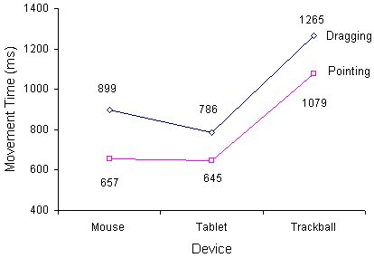
Although the degradation over tasks was significant (F_2,10 = 10.43, p < .005), this was largely due to the mouse. The degradation for the trackball was the same as for the mouse-tablet mean (F_1,11 = 0.03, n.s.), while the degradation was significantly greater for the mouse than for the tablet (F_1,11 = 22.56, p < .001). (Since the tablet-to-trackball lines are nearly parallel in Figure 19, it is concluded further that the tablet vs. trackball differences over tasks were not significant while the mouse vs. trackball differences were.)

The hypothesis that movement time is independent of device or task (H5, see p. 71) is rejected. Regardless of task, performance is slower using a trackball than a mouse or tablet-with-stylus. Furthermore, within devices, drag-select tasks take longer than similar point-select tasks. The mouse and tablet are comparable for point-select tasks, but the mouse is slower than the tablet for drag-select tasks. The latter point is important in considering the case for tablet-with-stylus input vs. mouse input. In the design of interactive systems emphasizing State 2 actions, evidence suggests that the tablet-with-stylus is better than the mouse or trackball.

6.2.6 Errors

An error was defined as selecting outside the target while pointing, or relinquishing the object outside the target while dragging. The grand mean for error rate (adjusted) was 6.2%. Error rates for pointing were low, with means of 2.8% for the mouse, 3.6% for the tablet, and 3.3% for the trackball. However, in the case of dragging, error rates were considerably higher, with means of 9.8% for the mouse, 12.3% for the tablet, and 15.8% for the trackball (see Figure 20).

Figure 20. Percentage errors by device and task

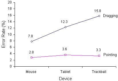
There was a significant main effect for task, with the dragging task yielding many more errors than the pointing task (F_1,11 = 45.28, p < .001). In addition, there was a significant main effect for device (F_2,10 = 7.25, p < .05). Error rates were higher for the trackball than for the mouse-tablet mean (F_1,11 = 9.37, p < .05), and, in turn, higher for the tablet than for the mouse (F_1,11 = 4.83, p < .05). The latter effect tends to counter the advantage of the tablet over mouse cited on the movement time criterion. (A comparison based on the combined effect on movement time and error rate is reported in the next section using IP.)

Although the device-by-task interaction was significant (F_2,10 = 11.22, p < .005), this was due to the trackball. The increase in errors across tasks was significantly greater for the trackball than for the mouse-tablet mean (F_1,11 = 24.64, p < .001); however, the increase for the tablet-with-stylus was comparable to that for the mouse (F_1,11 = 3.44, ns).

The hypothesis (H7) that error rate is independent of device or task is also rejected. Drag-select tasks yield more errors than point-select tasks. Across devices, error rates are about the same for point-select tasks; however, during dragging, the trackball has a higher error rate than the tablet-with-stylus which, in turn, has a higher error rate than the mouse.

6.2.7 Index of Performance

Although IP in the summary tables was calculated, for consistency, using Fitts' technique (see Table 1), the tests for main effects and interactions used IPs calculated with the Shannon formulation and the effective target width. These are felt to be the most representative measures of IP. Furthermore, IP was calculated using the direct method rather than linear regression. Although the latter measures are of greater importance in performance modeling (since they are taken directly out of the prediction equations), to use them in an analysis of variance is to ignore that portion of the variation accommodated by the intercept coefficient. (The different methods of obtaining IP are compared later.)

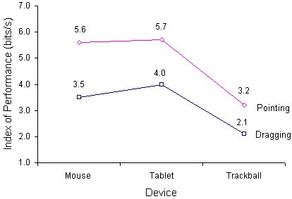
The grand mean for IP was 4.0 bits/s with means for the mouse, tablet, and trackball respectively of 5.6, 5.7, and 3.2 bits/s during pointing and 3.5, 4.0, and 2.1 bits/s during dragging (see Figure 21). There were significant main effects for device (F_2,10 = 133.10, p < .001) and task (F_1,11 = 302.79, p < .001), and a significant device-by-task interaction (F_2,10 = 77.28, p < .001).

Figure 21. Index of performance by device and task. (IP = ID / MT ; ID = log₂(1 + A / W_e))

The index of performance was significantly lower for the trackball than for the mouse-tablet mean (F_1,11 = 266.86, p < .001), and, in turn, slightly lower for the mouse than for the tablet (F_1,11 = 5.46, p < .05).

The degradation over tasks was less for the trackball than for the mouse-tablet mean (F_1,11 = 108.98, p < .001), and, in turn, less for the tablet than for the mouse (F_1,11 = 11.68, p < .01). Although, taken alone, this bodes well for the trackball, a contributing factor was the generally low IP for the trackball in both tasks.

The hypothesis that the rate of information processing is independent of device or task (H8) is rejected. For each device tested, IP is higher for point-select tasks, than for drag-select tasks. Across devices, the trackball has a lower IP than the mouse-tablet mean regardless of task. The mouse and tablet-with-stylus have similar IPs while pointing; but IP during dragging is higher for the tablet-with-stylus than for the mouse. Since IP is based on movement time and error rate, the conclusion made with respect to the movement time criterion is strengthened: In direct manipulation systems employing State 1 and State 2 transactions, the tablet-with-stylus performs better than the mouse or trackball.

6.2.8 Fit of the Model

The data in Table 9 and Appendix B were entered in regression analyses and tests of correlation using MT as the dependent variable and ID (computed using the Shannon formulation and using W_e(SD )), as the criterion variable. The results are shown in Table 10.

Table 10
Correlation and Regression Analyses for Experiment 1

Device	Task	r a	SE b (ms)	Regression Coefficients
				Intercept, a (ms)	Slope, b (ms/bit)	IP c (bits/s)
Mouse	Pointing	.9902	41	-107	223	4.5
	Dragging	.9921	38	135	249	4.0
Tablet	Pointing	.9876	40	-55	204	4.9
	Dragging	.9925	35	-27	276	3.6
Trackball	Pointing	.9809	78	75	300	3.3
	Dragging	.9226	190	-349	688	1.5
a n = 16, p < .001 b standard error of estimate c IP (Index of performance) = 1 / b

There were consistently high correlations between movement time (MT ) and the index of task difficulty (ID ) for all device-task combinations (r > .9000, p < .001). Performance indices (IP ), ranging from 1.5 bits/s to 4.9 bits/s, were less than those found by Fitts (1954) or Card et al. (1978), but were similar to those reported by Gillan et al. (1990), Jagacinski and Monk (1985), Kantowitz and Elvers (1988), and others. The rank order of devices changed across tasks. The tablet outperformed the mouse during pointing but not during dragging; however, the differences between the two devices were slight (0.4 bits/s). The trackball, third for both tasks, had a particularly low rating of IP = 1.5 bits/s during dragging.

Five of the intercepts were close to the origin (within 135 ms); however, a large, negative intercept appeared for the trackball-dragging condition (-349 ms). Although a negative intercept brings the possibility of a negative predicted movement time, this is unlikely because of the large slope coefficients. For example, under the latter condition, a negative prediction would only occur for ID less than 0.5 bits.

The standard error of estimate (SE ) is included in Table 10 to establish confidence intervals for predictions (see Glass & Hopkins, 1984, 126). For example, the predicted time to complete a dragging task with the mouse is

MT = 135 + 249 ID,

(25)

where ID is calculated using the Shannon formulation. From this, a task with ID = 5 bits should take 135 + 249(5) = 1380 ms. With SE = 38 ms, the 95% confidence interval is the predicted time plus or minus 2 × SE = 2 × 38 = 76 ms; that is, between 1304 ms and 1456 ms. Since the SEs were considerably lower for the mouse or tablet-with-stylus than for the trackball, the prediction equations for the latter device are of less practical value, particularly for dragging operations.

The poor performance of the trackball during dragging can be explained by noting the extent of muscle and limb interaction required to maintain State 2 motion and to execute state transitions. The button on the trackball was operated with the thumb while the ball was rolled with the fingers. It was particularly difficult to hold the ball stationary with the fingers while executing a state transition with the thumb: The interaction between limb groups was considerable. This was not the case with the mouse or tablet-with-stylus which afford separation of the means to effect action. Motion was realized through the wrist or forearm with state transitions executed via the index finger (mouse) or the application of pressure (tablet-with-stylus).

6.2.9 Comparison of Methods for Calculating IP

As illustrated at the beginning of this chapter (see Figure 17), the index of performance may be calculated numerous ways. In the previous two sections, for example, measures were obtained using the direct method (in tests of main effects and interactions) and using linear regression (in tests of the model). This is potentially troublesome if IP is to serve as a reliable statistic for device-task comparisons.

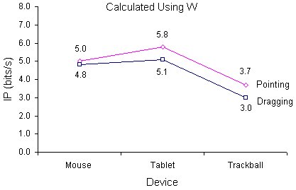
We begin our comparisons by introducing a third set of measures. In light of the point raised in Chapter 4 (that across-study comparisons are hampered by the inconsistent treatment of errors; see p. 62), it is worth comparing the six performance indices in Table 10 with those obtained using the specified target width (i.e., without normalizing for spatial variability). Had the table been derived using W instead of W_e(SD ), the IP ratings for the mouse, tablet, and trackball respectively would have been 5.0, 5.8, and 3.7 bits/s during pointing and 4.8, 5.1, and 3.0 bits/s during dragging. Figure 22 highlights the differences in plots of IP vs. device and task using (a) the specified target width (W ), as just cited, and (b ) using W_e(SD ) as given in Table 10.

(a)
(b)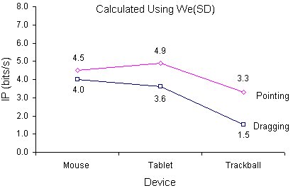
Figure 22. Index of performance by device and task (a) using W and (b) using W_e. (IP = 1 / b, from MT = a + b ID ; ID calculated using the Shannon formulation)

Before reviewing the merits or deficiencies in each method, a brief summary of the three methods presented thus far is in order. Figure 17 can assist in identifying each of the methods. The common thread is the use of adjusted data and the Shannon formulation for ID. The plots differ by the use of the direct method vs. linear regression (Figure 21 vs. Figure 22b) or by the use of W vs. W_e(SD ) (Figure 22a vs. Figure 22b).

First, a comparison is drawn between IPs obtained using the specified target width (W ) vs. the effective target width (W_e(SD )). In comparing Figure 22a with Figure 22b, the use of normalized values (a) reduced the IP ratings on the whole, (b) increased the spread of values, and (c) changed the rank order of devices across tasks. On point (a), reduced IPs also appeared in the re-analysis of Fitts' tapping experiments under the same conditions (that is, W_e(SD ) was substituted for W ; see Table 2). By no means is the drop in IP a bad sign. Improving the accuracy of the measurement is the goal, rather than achieving a specific, or high, value.

Point (b) — the increased spread in the normalized data — is particularly important in furthering the argument for normalizing for spatial variability before comparing performance measures. Normalizing tends to increase the sensitivity of the IP measures, teasing performance differences out of raw data.

This is evident in Figure 22 where the trackball's poor showing turned to dismal when the high error rate was also considered. Point (c) illustrates that device rankings based on IP are sensitive to the method of calculating IP.

A comparison of the direct and linear regression methods of calculating IP is also in order. Figure 22b contains IPs obtained from the regression line slopes (IP = 1 / b ) while Figure 21 contains IPs obtained by direct calculation (IP = ID / MT ). Both figures used the Shannon formulation and W_e(SD ). The device and task main effects reported using the measures in Figure 21 agree with the trends in Figure 22b; however, the device-by-task interactions are reversed in the two figures. In Figure 21, degradations over tasks were least for the trackball, and greatest for the mouse. The opposite pattern appears in Figure 22b. Since the IPs in Figure 22b were taken from the regression equations in Table 10, the intercepts should also be considered. It is felt that IPs taken from regression equations are not a reliable performance measure unless the intercepts are close to zero or reflect a systematic effect independent of IP. This is not the case here. Since intercepts ranged from -349 ms to 135 ms in Table 10, they cannot be attributed to a component of the task, such as the terminating button push. It appears that random effects were greater than systematic effects.

In summary, it is felt that, taken alone, the IP measures most useful for device-task comparisons are those obtained using the Shannon formulation, using W_e(SD ), and using the direct method of calculation; that is, IP = ID / MT, where ID = log₂(1 + A / W_e(SD )). The measures in Figure 21 fit this description.

6.2.10 Model Comparisons

As with the earlier model comparisons, the Welford formulation consistently yielded correlations between those obtained using the Fitts and Shannon formulations. The test for significant differences between models, therefore, proceeded only for the Fitts vs. Shannon formulations. Each of the six device-task conditions was entered in two model comparisons: one using W in the calculation of ID and one using W_e(SD ). The results in Table 11 show that the Shannon model correlated higher than the Fitts model for all 12 data sets; however, statistical significance in the difference using Hotelling's t test (two-tailed) was achieved only twice (p < .05).

Table 11
Comparison of Fitts and Shannon models for Experiment One

Device	Task	ID Range a		Correlations by Model			Higher	Hotelling's t test b
		Low	High	Fitts	Shannon	Inter-Model		t	p
*** Calculated using W ***
Mouse	Pointing	1	7	.9866	.9920	.9966	Shannon	1.88	-
	Dragging	1	7	.9862	.9914	.9966	Shannon	1.78	-
Tablet	Pointing	1	7	.9921	.9951	.9966	Shannon	1.29	-
	Dragging	1	7	.9830	.9905	.9966	Shannon	2.52	.05
Trackball	Pointing	1	7	.9673	.9749	.9966	Shannon	0.99	-
	Dragging	1	7	.9673	.9749	.9966	Shannon	1.54	-
*** Calculated using We(SD) ***
Mouse	Pointing	1.92	6.94	.9887	.9902	.9986	Shannon	0.72	-
	Dragging	1.41	6.29	.9675	.9921	.9976	Shannon	1.96	-
Tablet	Pointing	1.99	6.62	.9869	.9876	.9988	Shannon	0.34	-
	Dragging	1.66	6.05	.9886	.9925	.9980	Shannon	1.92	-
Trackball	Pointing	1.54	6.75	.9778	.9809	.9980	Shannon	0.91	-
	Dragging	1.06	4.10	.9038	.9226	.9968	Shannon	2.54	.05
a calculated using Fitts' formulation b two-tailed text, n = 16, df = 13

As with the earlier model comparisons, it is worth examining the effect of normalizing target width on the difference between models. In all cases, using the effective target width reduced the range of IDs. Thus, the hypothesized improvement in the correlations using the Shannon formulation is countered, at least partly, by two influences: (a) the tendency for correlations to drop when a sample is drawn from a restricted range in a population, and (b) the reduced differences in the two formulations when low values of ID are poorly represented. In four of six cases in Table 11, the t statistic dropped when W_e(SD ) was introduced in the calculation of ID. The two cases in which the t statistic increased (mouse-dragging & trackball-dragging) are perhaps a sign of the tendency for W_e(SD ) to increase the correlation due to the theoretical benefits in normalizing target width.

The upper extent of the IDs dropped considerably (from 7 bits to 4.10 bits) when using W_e(SD ) under the trackball-dragging condition. This was due to the extremely large variation in x coordinates pushing the effective target width up, thereby reducing the effective ID. Error rates were over 14% for all trackball-dragging conditions above 3 bits of difficulty. In essence, subjects were not performing the tasks specified, but were realizing tasks with a much lower ID.

The hypothesis that the Fitts, Welford, and Shannon models are the same (H1) remains tenable based on Table 11. The present analysis provides only moderate support that the Shannon model accounts for observations better than the Fitts model. Nevertheless, along with the model comparisons presented earlier (Table 3 & Table 4), Table 11 adds strength to the claim that the Shannon formulation is empirically superior to the Fitts formulation. Since the Welford model yielded correlations between those for the Fitts and Shannon models, further comparisons were not undertaken.

It is felt, in retrospect, that a slightly different experimental procedure may be needed before the differences between models stand out. In particular, a higher error rate must be attained for small IDs. Subjects would require feedback and incentive to speed up and commit more errors when tasks are easy. This, however, changes the nature of the experiment. The reckless behaviour that would ensue is remote from user input tasks on computers. An experiment focusing specifically on the model differences could pursue this further; however, since the present experiment also addressed the role of device and task, it would have been misguided to introduce such a procedure.

The hypothesis that correlations are the same using the effective target width vs. the specified target width (H2) also remains tenable based on Table 11. In retrospect, the benefits in using the effective target width are not so much an improved fit, but that resulting measures facilitate comparisons across experimental factors and, as noted in Chapter 4, across studies. Arguably, the adjustment (or maintaining a consistent error rate) is essential for an "apples with apples" comparison of performance measures.

6.3 Experiment 2

6.3.1 Adjustment of Data

A Newman-Keuls test using movement time and error rate as criterion variables showed no significant differences in the 15 session means for Experiment 2. Therefore, all the data were entered in the test for outliers. As in Experiment 1, trials with selection coordinates more than three standard deviations from the mean were eliminated; however, for Experiment 2, both the x and y coordinates were tested. Of 14,040 total trials, 42 (0.3%) qualified as outliers and were removed.

An additional criterion was introduced. Occasionally, subjects seemed confused about when timing had started on a trial. They returned to the start circle and waited even though timing had begun. Upon realizing this, they proceeded as usual. Such trials had uncharacteristically long movement times; and, so, a five second limit was set. This criterion was met by one trial in Experiment 2 (and by four trials in Experiment 3).

6.3.2 Approach Angle

Approach angle was the only factor fully crossed with other factors; therefore, an analysis of variance was applied only to the main effect of approach angle on the dependent measures of movement time and error rate.

Trials were timed from the cursor leaving the start circle to the button- down action at the target. The grand mean for movement time was 743 ms. Moves along the horizontal and vertical axes were about the same (733 and 732 ms) while moves along the diagonal axis took 4% longer (MT = 764 ms, F_2,22 = 23.86, p < .001). Although the statistical significance in the difference implies that hypothesis H3 can be rejected, the practical significance of a 4% difference is probably slight.

The grand mean for error rate was 4.6%, with means along the horizontal, diagonal, and vertical axes of 3.9%, 5.1%, and 4.7% respectively. Again, statistical significance was achieved (F_2,22 = 4.33, p < .05) and, so, hypothesis H4 can be rejected.

These results were as expected. Although the differences should be noted, a slightly different movement time or error rate does not give one model a significant or unfair advantage over the others since a range of short-and-wide and tall-and-narrow targets were used.

6.3.3 Fit of the Model

The main objective in this experiment was to compare several models for target width when the approach angle varies. Five models were tested:

Model	Target Width
status quo W+H W×H smaller-of W '	horizontal extent (W ) sum of width and height area smaller of width or height (SOWH ) width along line of approach

Each model was entered in a test of correlation and linear regression using the Fitts and Shannon formulations for index of difficulty. The results are given in Table 12.

Table 12
Comparison of Models for Target Width

Model for Target Width a	ID Range (bits)		r b	SE c (ms)	Regression Coefficients
	Low	High			Intercept, a (ms)	Slope, b (ms/bit)	IP (bits/s)
*** Fitts Formulation, ID = log2(2A / W) ***
SOWH	2.00	6.00	.945	66	196	142	7.0
W'	1.00	6.00	.9378	71	340	129	8.3
W+H	0.42	4.42	.8888	94	482	146	6.9
W×H	−1.00	5.00	.8714	101	559	114	8.8
W	1.00	6.00	.8066	122	419	107	9.4
*** Shannon Formulation, ID = log2(A / W + 1) ***
SOWH	1.58	5.04	.9501	64	230	166	6.0
W'	1.00	5.04	.9333	74	337	160	6.0
W+H	0.74	3.54	.8755	99	402	218	4.6
W×H	0.32	4.09	.8446	110	481	173	5.8
W	1.00	5.04	.8097	121	409	135	7.4
a W = target width, H = target height, SOWH = smaller of W or H, W' = width along line of approach b n = 78, p < .001 c standard error of estimate

The correlations were above .8000 (p < .001) in all cases. The smaller-of model (SOWH ) had the highest correlation and the lowest standard error, while the status quo model (W ) had the lowest r and the highest SE. Correlations and SEs for the W' model were comparable to those for the smaller-of model. On the whole, performance indices (IP ) were several bits/s higher than for the mouse-pointing condition in Experiment 1. This agrees with observations made by others that discrete tasks yield higher IPs than serial tasks. The intercepts were all positive with the smaller-of model yielding the intercept closest to the origin. The highest IP was 9.4 bits/s for the status quo model using Fitts' formulation. This is close to the value of 10.4 bits/s obtained by Card et al. (1978).

Comparing the correlation and regression coefficients between the Fitts and Shannon formulations, there was no dramatic or unanticipated difference. As before, the Shannon formulation yielded a lower IP than the Fitts formulation (cf. Table 2 & Table 12). Because of the different substitutions for target width, the range of IDs for each model differed. Furthermore, for each model the range lessened using the Shannon formulation. This in itself would tend to reduce the correlations in the latter case.

The highest correlation in Table 12 was for the smaller-of model for target width combined with the Shannon formulation for ID. Therefore, using a mouse the predicted time (ms) to point to and select a rectangular target, regardless of approach angle, is

MT = 230 + 166 ID.

(26)

With SE = 64 ms, there is 95% confidence that the time to complete a task rated at 5 bits of difficulty is 230 + 166(5) ± 2(64); that is, between 932 ms and 1188 ms.

Equations 26 and 25 are the best prediction equations emerging from this research for predicting the time to complete pointing tasks or dragging tasks using the mouse. We shall meet these again in Experiment 3.

6.3.4 W_e in Two Dimensions

There are several possible ways to calculate the effective target width for two-dimensional target acquisition tasks. By a status quo approach, the calculation could proceed as before, using the standard deviation in selection coordinates along the x axis (W_ex). Since approach angle varied, a reasonable alternative is to use the standard deviation in the two-dimensional displacement of selections from target centre (W_exy). (This was discussed on p. 28.) A smaller-of model suggests that W_ex or W_ey should be substituted, as appropriate. Finally, a W' view would use the standard deviation in the displacements measured parallel to the approach axis. Table 13 compares each of these methods, showing the range of "effective" IDs (calculated using the Shannon formulation), the MT-ID correlation, the standard error of estimate, and the regression coefficients.

Table 13
Comparison of Methods for Calcualating W_e in Two Dimensions

Model	Effective Target Width a	ID Range (bits)		r b	SE (ms)	Regression Coefficients
		Low	High			Intercept, a (ms)	Slope, b (ms/bit)	IP (bits/s)
Status quo	Wex	1.00	5.22	.8528	107	300	160	6.3
	Wexy	1.56	5.61	.8757	99	225	175	5.7
Smaller-of	Wex or Wey	1.59	5.28	.9040	88	207	166	6.0
W'	We'	1.00	5.15	.9071	86	290	170	5.9
a see text for method of calculation b n = 78, p < .001

Since error rates were close to 4%, dramatic differences were not expected for models derived using the effective target width. The regression coefficients are similar to those in Table 12, as are the range of IDs for each model. More is gained by comparing the methods to one another. The correlation was slightly higher using the two-dimensional displacement (W_exy) vs. the one-dimensional displacement (W_ex); however, further increases in r were obtained using the smaller-of (W_ex or W_ey) and W_e' models. The fact that the W_e' model yielded the highest r may follow from the theoretical benefits in maintaining the model's inherent one-dimensionality. Nevertheless, overall, the highest correlation was obtained using the smaller-of model without normalizing target width (Equation 26; see Table 12).

6.3.5 Model Comparisons

The ranking of correlations in Table 12 and Table 13 suggests that the status quo model is in trouble for two-dimensional target acquisition tasks. Pair-wise comparisons of models were undertaken using Hotelling's t test, as before. The difference between the correlations was not significant for the status quo model vs. W+H models (t = 2.00, df = 75, n.s.), or for the status quo vs. W×H models (t = 0.91, df = 75, n.s.). Therefore, the W+H and W×H models were excluded from further pair-wise comparisons. The correlations for the status quo, smaller-of, and W' models are compared in Table 14. As evident, the correlation was significantly higher for the smaller-of and W' models than for the status quo model (p < .001). Furthermore, the smaller-of and W' models did not differ significantly from each other (p > .05).

Table 14
Test for Significant Differences Between Models

Comparison of Models Target Width a		Correlations of ID with Movement Time b			Hotelling's t test c
1st Model	2nd Model	1st Model	2nd Model	Inter-model	t	p
SOWH	W'	.9501	.9333	.8502	1.32	-
SOWH	W	.9501	.8097	.7881	6.31	.001
W'	W	.9333	.8097	.6992	4.86	.001
a W = width, SOWH = smaller of W or H, W' = width of target on line of approach b p < .001, ID computed using Shannon formulation c two-tailed test, n = 78, df = 75

An initial conclusion, therefore, is that the smaller-of and W' models are empirically superior to the status quo model. As noted earlier, the W' model is theoretically attractive since it retains the one-dimensionality of the model. In a practical sense, the smaller-of model is appealing because it can be applied without consideration of approach angle. This is also true of the status quo model, but not of the W' model.

Since these results are potentially important to researchers interested in applying Fitts' law to two-dimensional target acquisition tasks, discussions should continue in more detail. The role of target height and approach angle varies in each model and therefore the comparisons may not be equitable. For example, in the status quo model, H and Θ_A do not participate. Is this a strength or a weakness in the model? In one sense, it is a strength, because fewer parameters implies greater generality and ease in application. On the other hand, if an additional parameter is shown to effect the dependent variable of interest, and the effect is to degrade the performance of the model in comparison to another, then the absence of the extra parameter must be taken as a weakness. Of course, the range of conditions tested must be representative of the application. The present experiment measured the time to acquire rectangular targets in two-dimensional tasks. The levels of factors were not unlike those in interactive computer graphics systems, with the possible exception of text selection, where the majority of targets are short-and-wide. (The limited case of text selection is discussed shortly.)

With respect to generality, the same argument can be made in comparing the smaller-of and the W' models. While the latter can be applied only with knowledge of A, W, H, and Θ_A, the smaller-of model only uses A, W, and H. This is both a strength and a potential weakness in the smaller-of model. It is possible that angles between 0° and 45° , for example, may yield variations in movement time more consistent with predictions in a W' model than a smaller-of model. This remains to be tested. Nevertheless, the generality afforded by applying the smaller-of model with one less parameter is noteworthy.

6.3.6 Parametric Analysis

A parametric analysis was undertaken to compare the status quo and smaller-of models using the Fitts and Shannon formulations. The results are shown in Figure 23. The graphs show the predicted movement time as a function of target width using the formula MT = a + b ID, where ID is a function of W, H, and A. Target height (H ) was held constant at 1 unit while W and A varied from ⅛ to 8 units by powers of two. In reality, a series of graphs should be presented, each corresponding to a unique value for H. Each graph in the series would be identical for the status quo model because H does on participate; however, each smaller-of graph would have an "elbow" where the predicted movement time levels off. As shown in Figure 23, the elbow occurs at W = H.

Figure 23. Parametric analysis comparing the "status quo" and "smaller of" models

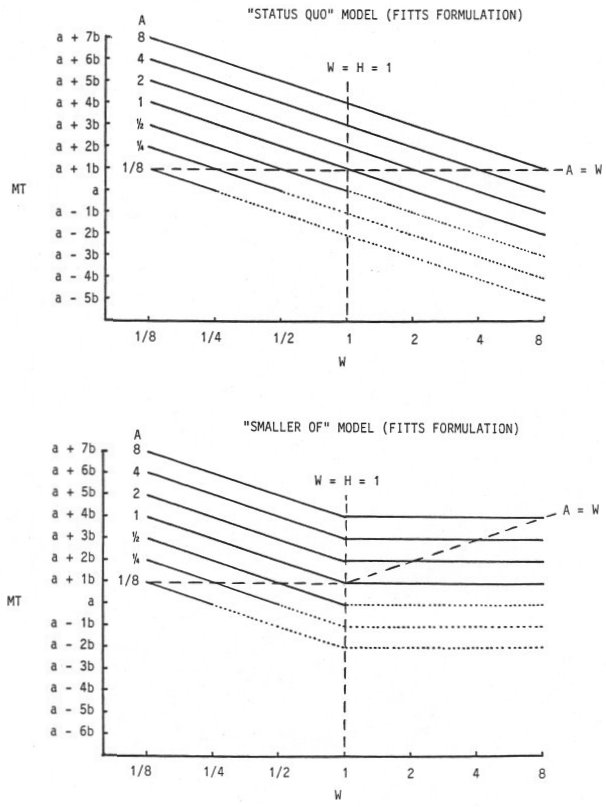
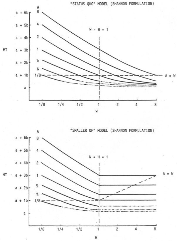
Solid lines in Figure 23 represent equal amplitudes. The vertical and horizontal dashed lines divide the graphs into four regions on either side of W = H and A = W. Short-and-wide targets are on the right, tall-and-narrow targets are on the left. The regions below A = W are potentially troublesome because A < W. Problems begin at A < W / 2 (or A < H / 2) because the task is meaningless for some approach angles. The dotted lines replace solid lines under conditions where the starting position is inside the target regardless of approach angle. Obviously, such conditions cannot occur. The solid lines show conditions which may be reasonably expected, although limitations exist. For example, targets cannot be approached at Θ_A = 0° when A < W / 2. Nevertheless, A < W / 2 is a perfectly reasonable condition for other approach angles. A typical example is selecting a short-and-wide target, such as a word, from above or below at close range: The target may be substantially wide in comparison to the distance.

Several observations follow from Figure 23. For a given A (where A > H ), the predicted movement time using the status quo model and the Fitts formulation decreases without limitation — and eventually becomes negative — as W increases. This is a problem. Surely, a finite amount of time is needed to cover the distance to the target, regardless of the width! This is precisely what is predicted in the smaller-of model when W exceeds H: The predicted movement time levels off and depends only on A.

Using the Shannon formulation, the outcome is similar. Predicted movement time with the status quo model continually decreases but approaches the intercept, a. With the smaller-of model, predictions bottom out when W exceeds H, but the limit increases with A. Although there may be a slight improvement in using the Shannon formulation, the differences between the models for target width are clearly more dramatic than those between formulations.

The comparison is now continued using the experience in the present experiment. For each target height condition, the predicted and observed points for the conditions tested were plotted for the status quo and the smaller-of models. The points were placed on contour lines for each target amplitude condition. Fitts' formulation was used only because the graphs were easier to render. For convenience, the observed points were labeled A, B, C, etc. The results are shown in Figure 24.

Figure 24. Plot of predicted and observed MTs in Experiment 2

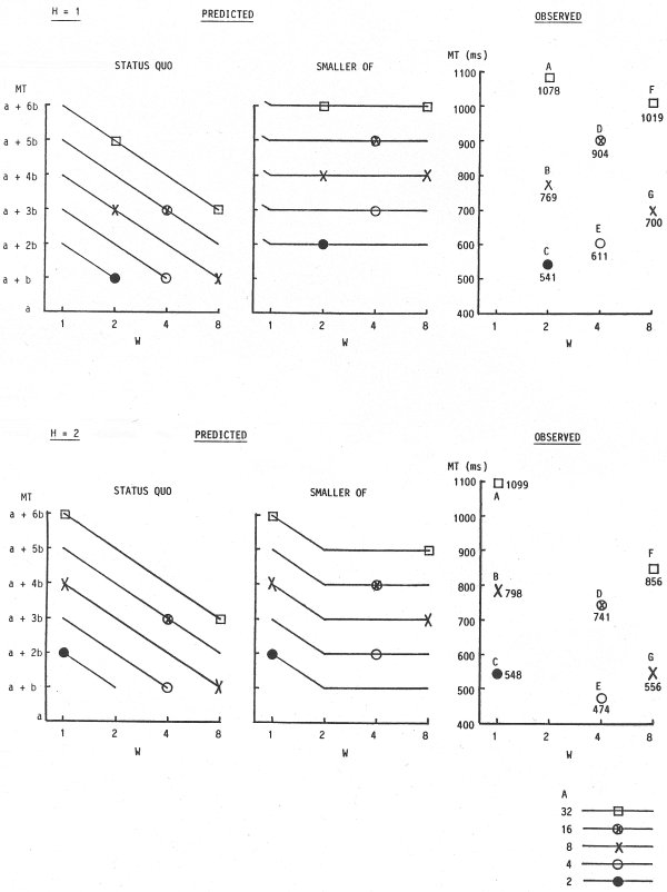
For the status quo model, all points fall on a series of negatively sloped lines for different amplitude conditions. For the smaller-of model, the position of the points depends on H. For H = 1, all the points tested fall on the flat line segments for the smaller-of model; thus, predicted movement times differ considerably between models. For example, consider the three-point sequences B-D-F and C-E-G. A line through each triplet in the observed data slopes upward. The similarity with predictions in the smaller-of model is remarkable. Furthermore, the magnitude of the change approaches the predicted increase of 2b ms for each triplet. Since the regression line slope was 142 ms/bit for the smaller-of model using the Fitts formulation (see Table 12), predicted increases were 284 ms for each triplet. Observed increases were 250 ms for the B-D-F triplet and 159 ms for the C-E-G triplet.

Support for the smaller-of model in Figure 24 is by no means unanimous. Again examining the H = 1 condition, predicted slopes for the point pairs A-F and B-G are negative by the status quo model and zero by the smaller-of model. Although observations agree with the status quo model, the support is less than resounding. Predictions call for a decrease of 2b ms, or 214 ms based on the regression line slope. Observed decreases were 59 ms for the A-F pair and 69 ms for the B-G pair.

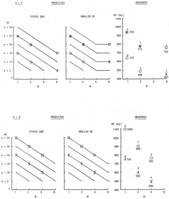
Since square targets were not used, no point tested falls on the elbow of the contour lines. For H = 2 and H = 3, however, a mixture of short-and-wide and tall-and-narrow targets were used. While little is gained in itemizing the supporting trends in Figure 24, observations in general support the smaller-of model. The H = 8 condition is rather uninteresting because the models do not differ: The width of the target was always the smaller of W or H.

Note that the subset of conditions with H = 1 provides the strongest support for the smaller-of model and uses short-and-wide targets. This is important in establishing the viability of the smaller-of model in the limited case of text selection where short-and-wide targets are the norm. In fact, the case of H = 2 is the closest to text selection because the H:W ratio of single characters is generally about 2:1. Thus, when H = 2 the conditions W = 1, 4, and 8 units parallel those for words of 1, 4, and 8 characters respectively. Had the present experiment included conditions with, for example, W = 16 or 32 units, the support for the smaller-of model probably would have been stronger (based on the trends in Figure 24). For further evidence, we need only to examine the observations of Gillan et al. (1990), who used conditions of W = 1, 5, 14, and 26 characters. The contour lines in Figure 23 and Figure 24 for the smaller-of model are remarkably similar to those in Figure 13 (see p. 68).

6.3.7 The W' Model

The W' model, although the most difficult to apply, performed as well as the smaller-of model in Table 12. An assumption in the model is that subjects move toward the centre of the target. No doubt, optimization would follow under extreme conditions, such as moving toward a very wide target at close range. If the starting point is below at a 45° angle from the target centre, for example, movement distances could be reduced by advancing along a more direct path, closer to 90°. Such extremes were not tested. To prevent biasing the comparisons for any one model, the experiment fully crossed the three approach angles with all amplitude-width-height conditions; thus, the minimum amplitude for each condition could be applied at each approach angle. Optimization trends were investigated by calculating the actual amplitudes and approach angles for all 78 conditions. As expected, subjects optimized moves the most for the extreme short-and-wide and tall-and-narrow targets. Under the condition W = 8, H = 1, A = 8, and Θ_A = 45°, means for the actual amplitude and approach angle were 7.1 units and 36.9° respectively. Under the opposite width-height extreme (W = 1, H = 8, A = 8, and Θ_A = 45°) means were 7.3 units and 50.4°. These figures represent the greatest deviation of output from input. For the vast majority of conditions, actual amplitudes and angles were remarkably close to the specified conditions. Analyses using "effective" or actual measures for A and Θ_A were not pursued further.

When non-rectangular targets are used, the smaller-of model is in trouble, whereas the W' model can be applied in the usual way. Nevertheless, it is easy to imagine odd-shaped targets without an obvious "centre". The W' model may yield unreasonably large or small estimates for target width in some instances. The area model (W×H ) has some intuitive appeal in this case. One can imagine reducing an odd-shaped target to a minimum-circumference shape – a circle – having the same area. The W×H model would substitute the area for W, while the W' model would substitute the diameter.

To conclude, the results in Table 12 and Table 14 lead to the rejection of the hypothesis (H5) that MT-ID correlations are independent of several models for target width. In two-dimensional target acquisition tasks, the choice of target width in the calculation of a task's index of difficulty plays a critical role in the accuracy of the model. Consistently using the horizontal extent of a target as its "width" (as consistent with the status quo view) weakens the model and leads to inaccurate and sometimes erroneous predictions. Two models performed significantly better than the status quo model. The first — the W' model — substitutes for W the extent of the target along an approach vector through the centre. This model is theoretically attractive since it retains the one dimensionality of Fitts' law; however, the approach angle (as well as the width, height, and amplitude) must be known a priori. The second — the smaller-of model — substitutes for W either the width or height of the target, whichever is smaller. This model is easy to apply, but is limited to rectangular targets, unlike the W' model. Both models, in tests of correlation, performed significantly better than the status quo model; however, no difference was detected between them.

6.4 Experiment 3

The criteria for adjusting data from Experiment 2 were also applied in Experiment 3. No significant differences were found in the fifteen session means. Of 18,360 total trials, 378 (2.1%) qualified as outliers and were removed. An additional 4 trials were dropped because movement time exceeded 5 seconds.

A goal of Experiment 3 was to explore the possibility of taking a derived Fitts' law model and applying it in subsequent designs. A simplistic opportunity for doing this was afforded by applying the models built in Experiments 1 and 2 on observations in Experiment 3. Approach angle varied in Experiment 3; but this was only of concern in the pointing phase of a task since dragging was consistently left-to-right.

Movement time for the initial point operation (MT_P) was timed from the cursor leaving the start circle to the button-down action at the pick-up region on the left of the target (see Figure 16). Movement time for dragging (MT_D) was timed from the end of the initial point operation to the button-up action at the drop region on the right. The mean time to complete moves was 633 ms (SD = 213 ms) for the pointing phase of tasks followed by 827 ms (SD = 226 ms) for the dragging phase. Mean error rates were 1.8% (SD = 3.7%) for pointing and 4.2% (SD = 6.0%) for dragging.

Although 102 unique conditions were tested (see Table 8), the data were aggregated by conditions unique to each of the pointing and dragging phases of the tasks. Aggregating by point-amplitude, width, height, and angle left 54 conditions for the pointing analysis. Aggregating by drag-amplitude, width, and height left 15 conditions for the dragging analysis. Regressing MT_P (ms) on ID, where ID = log₂(1 + A / SOWH ), yielded

MTP = 177 + 169 ID

(27)

with r = .9637 (p < .001) and SE = 54 ms. Regressing MT_D (ms) on ID, where ID = log₂(1 + A / W ), yielded

MTD = 345 + 198 ID

(28)

with r = .9711 (p < .001) and SE = 54 ms. The high correlations in these analyses are, in themselves, support for the hypothesis (H9) that point-drag-select tasks can be modeled as two separate Fitts' law tasks, each with its own prediction equation.

A scatter plot of points is shown in Figure 25a for pointing and Figure 25b for dragging. Each point plotted was derived from the mean of more than 300 observations. The dashed lines apply to Experiment 3, with the range of conditions delimited on the left and right, and the 95% confidence intervals (on observed points) delimited on the top and bottom. The solid lines show the 95% confidence intervals predicted from the models derived in Experiment 2 (Equation 26, pointing) and Experiment 1 (Equation 25, dragging).

Figure 25. Predicted and observed 95% confidence intervals for a point-select task. The pointing phase (a) and dragging phase (b) were analyses separately

Since Experiments 2 and 3 were conducted together, it is not surprising that the solid and dashed lines are more similar in Figure 25a than in Figure 25b. Of the 54 aggregate points for pointing, four (8.9%) were below the predicted 95% confidence band; none was above. Of the 15 aggregate points for dragging, eight (53.3%) were above the predicted 95% confidence band; none was below.

The use of a model derived from a serial dragging task (Equation 25 from Experiment 1) may be inappropriate for the dragging phase of a discrete point-drag-select task. It is evident in Figure 25b that Equations 25 and 28 have very different intercepts and slopes. The regression coefficients and standard errors (SEs ) are summarized in Table 15 for the four equations in question.

Table 15
Comparison of Four Regression Equations

Equation	Experiment	r a	SE (ms)	Regression Coefficients
				Intercept, a (ms)	SE (ms)	Slope, b (ms/bit)	SE (ms/bit)	IP (bits/s) b
*** Pointing ***
26	2	.9501	64	230	21	166	6.2	6.0
27	3	.9637	54	177	19	169	6.5	5.9
*** Dragging ***
25	1	.9921	38	135	26	249	8.4	4.0
28	3	.9711	54	345	36	198	13.0	5.1
a p < .001 b IP = 1 / b Note: Eq. 25 is from Exp. 1, Eq. 26 is from Exp. 2, and Eq 27 & 28 are from Exp. 3

Since the correlations were very high (r > .9000, p < .001), it is not surprising that standard errors throughout were low. It appears the regression equations were all highly representative of observations in the respective tasks. More relevant, however, is whether or not the two pointing equations are "the same", and whether or not the two dragging equations are "the same". The standard error for each regression coefficient is valuable for this comparison. First examining the two pointing equations with Equation 27 as the reference, the slope coefficients differ by (169 − 166) / 6.5 = 0.46 SEs. This is extremely close. The intercept in Equation 26, however, is 2.8 SEs higher than the intercept in Equation 27. The latter difference would only occur 0.5% of the time through random effects (with the assumption of normality); so, despite the insignificant differences in slopes, it cannot be assumed that the two prediction equations apply to the same underlying task. This may be attributable to the subtle differences in the task s (point-select vs. point-drag-select), or to the slightly different range of conditions tested (cf. Table 7 & Table 8). Despite efforts to make the conditions similar, duplicating the target width-height conditions from Experiment 2 in Experiment 3 would have produced some odd tasks (e.g., dragging a very short-and-wide box left-to-right).

The two dragging equations in Table 15 are quite different. Using Equation 28 as the reference, the slope is 3.9 SEs higher and the intercept 5.8 SEs lower for Equation 25. There are several possible sources of this disparity. First, Experiments 1 and 3 were conducted separately using different subjects. Second, the range of conditions was different. IDs ranged from 1 to 6 bits in Experiment 1 and from 1.8 to 5 bits in Experiment 3. Finally, the tasks were different. Equation 25 was derived from a serial dragging task, but was applied to data for the dragging phase of a discrete point-drag-select task. Yet, these tasks are similar enough that even greater disparities would probably arise if the derived models were applied to State 1 and State 2 actions on "real" interactive graphics systems, where an assortment of user actions arise. Tasks such as selecting words or blocks of text in a word processing environment, acquiring and manipulating icons, or selecting an item in a pull-down menu would severely test the generality of a model built in a research environment.

The present attempt to apply derived models to subsequent tasks illustrates the difficulty in adopting models such as Fitts' law to practical problems in interface design. Meeting the usual statistical tests for validity seems easy in comparison to the challenges in applying the model later. Expectations must be kept low. A statistically sound model will be accompanied by a small standard error of estimate; but confidence intervals will not be met unless the model was derived under conditions similar to the application.

6.4.1 Target Width in Dragging Tasks

One final, brief analysis is presented. Gillan et al. (1990) tested Fitts' law in dragging tasks and concluded that "dragging time in a point-drag sequence is under control of two features of a computer display: the dragging distance and the height of the text object" (p. 232). Two models were compared: one substituting the constant 0.5 cm for target width and another substituting target height, H. A higher correlation was found in the latter case, and this led to the conclusion above. It was pointed out in Chapter 4 (see p. 69) that the "target height" model was suspect because character width was positively correlated with character height; thus, as targets got higher, they also got wider. It is felt that Gillan et al. (1990) inadvertently confirmed the strength of the status quo model for one-dimensional tasks.

Since Experiment 3 included a balanced set of square, short-and-wide, and tall-and-narrow targets (see Table 8), H and W were uncorrelated. This permitted a valid test of Gillan et al.'s (1990) model against the status quo and smaller-of models. (The W' model is the same as the status quo model, in this case, because the approach angle was consistently 0°.)

Correlations for the status quo, smaller-of, and target height models respectively were .9711 (p < .001), .9688 (p < .001), and .6403 (p < .005). The poor showing of Gillan et al.'s (1990) model was fully anticipated. Since target height is measured perpendicular to the line of approach (in left-to-right dragging tasks), there is no reasonable basis for it to serve as target width in the model. Target height would have only a slight effect on movement time, since motion was one-dimensional along the horizontal axis. Therefore the top ranking for the status quo model (which is the same as the W' model in this case) was not surprising.