Field lines for electric fields

We calculate field lines for an electric field produced by a few charges by integrating the trajectories for positive probe charges. The fields are calculated by taking the gradient of the sum of the Coulomb potentials created by the fixed charges.

Suppose we have a single positive fixed charge of two units located at the origin, and two single negative charges elsewhere in the x-y plane. We will start the trajectories on a small circle surrounding the positive charge, and we will terminate them when they get too close to a negative charge, or when the speed reaches a very large value.

We work in simple units ( e =1, m =1)

> restart;

> with(plots):

Warning, the name changecoords has been redefined

> P1:=[-2,-3]; P2:=[3,1];

> Vpot:=(x,y)->2/sqrt(x^2+y^2)-1/sqrt((P1[1]-x)^2+(P1[2]-y)^2)-1/sqrt((P2[1]-x)^2+(P2[2]-y)^2);

We illustrate the potential by a contour diagram which shows equipotential lines (lines of equal potential energy). Think about topographic maps which display the height of mountains and depth of seas/ocenas to understand the diagram.

The field lines will cross these lines at right angles, as the gradient of the potential (which gives the electric field vector) is perpendicular to the equipotential contours.

> PL1:=contourplot(Vpot(x,y),x=-6..6,y=-6..6,axes=boxed,filled=true,coloring=[blue,red],grid=[40,40],contours=[-1,-0.8,-0.6,-0.4,-0.2,0.,0.2,0.4,0.6,0.8,1.,1.2,1.4,1.6,1.8,2.],scaling=constrained): display(PL1);

When calculating the electric field one has to understand that one differentiates the potential first, and then supplies the values of (x,y) at which one calculates the x- and y-components. This can be achieved either by differentiating the mapping Vpot, and then evaluating. Alternatively one would have to differentiate the expression Vpot(x,y) and subsequently substitute the values.

We make use of the operator D which differentiates mappings for two reasons: 1) it is more elegant; 2) we want to show how to use D with multivariate functions:

(note that the minus sign makes the display of Maple's answer look unpleasant)

> Ex:=-D[1](Vpot);

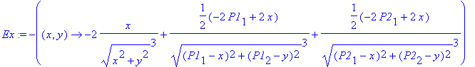
> Ey:=-D[2](Vpot);

To demonstrate where the electric field is strong we can make a contourplot of the magnitude of the electric field. No directional information is contained in this plot, but there should be an indication where we expect the field lines to be dense.

> PL2:=contourplot(sqrt(Ex(x,y)^2+Ey(x,y)^2),x=-6..6,y=-6..6,axes=boxed,filled=true,coloring=[white,red],grid=[40,40],contours=[0.2,0.5,1.,2.,5.,10.],scaling=constrained): display(PL2);

Which way does the field vector point?

> [Ex(0.2,0.),Ey(0.2,0.)];

To draw the field lines we step along the direction in which the electric field vector points. We start by choosing initial points on a circle around the positive charge at the center and pick 20 initial positions:

> r0:=0.2; r02:=r0^2; Nt:=20;

> phi:=i->(i-1)*2*Pi/Nt;

> Nmax:=1000; #the maximum number of points

> dt:=0.01;

> x_i:=r0*cos(phi(1)): y_i:=r0*sin(phi(1)): Rt:=[[x_i,y_i]]: for it from 1 to Nmax do: Fx:=Ex(x_i,y_i); Fy:=Ey(x_i,y_i); F_m:=sqrt(Fx^2+Fy^2); if dt*F_m>0.25 then dt:=dt/2 elif dt*F_m<0.1 then dt:=dt*2. fi; x_i:=evalf(x_i+dt*Fx); y_i:=evalf(y_i+dt*Fy); Rt:=[op(Rt),[x_i,y_i]]: if evalf((P1[1]-x_i)^2+(P1[2]-y_i)^2)<r02 or evalf((P2[1]-x_i)^2+(P2[2]-y_i)^2)<r02 or F_m>70. then break fi; od:

Now that we know that the calculation for one fieldline worked we can complete the loop:

> for j from 2 to Nt do: dt:=0.01; x_i:=evalf(r0*cos(phi(j))): y_i:=evalf(r0*sin(phi(j))): Rt:=[op(Rt),[x_i,y_i]]: for it from 1 to Nmax do: Fx:=Ex(x_i,y_i); Fy:=Ey(x_i,y_i); F_m:=sqrt(Fx^2+Fy^2); if dt*F_m>0.25 then dt:=dt*0.5 elif dt*F_m<0.1 then dt:=dt*2. fi; x_i:=evalf(x_i+dt*Fx); y_i:=evalf(y_i+dt*Fy); Rt:=[op(Rt),[x_i,y_i]]: if evalf((P1[1]-x_i)^2+(P1[2]-y_i)^2)<r02 or evalf((P2[1]-x_i)^2+(P2[2]-y_i)^2)<r02 or F_m>70. then break fi; od: od:

We can check the total number of points assembled into the list (all fieldlines in one list):

> nops(Rt);

> PL3:=plot(Rt,style=point,symbol=cross,view=[-6..6,-6..6],axes=boxed,scaling=constrained,color=black): display(PL3);

> display(PL1,PL3);

> display(PL2,PL3);

We note that the criteria to stop field lines are somewhat touchy:

If we step too quickly towards a charge where the field line is supposed to stop (i.e., dt is so large that we jump over the charge), we can create artificial lines that stop in 'mid-air'. We tried hard to recognize the vicinity of a strong increase in the field by:

a) adjusting the 'time'-step according to the size of the field

b) terminating if the field strength becomes large in addition to the vicinity criterion.

In a correct field line plot we have the following properties for electric field lines:

a) field lines originate in positive charges and terminate in negative ones;

b) field lines are perpendicular to equipotential contours

c) the density of field lines is indicative of the strength of the field.

Our plot has one deficiency (and increasing the number of points Nmax to 10,000 has resulted in excessive calculations without fixing the problem):

there is a field line escaping to 'infinity' in the top left of the graph, and apparently an incoming line is missing in the bottom left of the graph.

We are interested in demonstrating some real trajectories. The field lines indicate the acceleration that a particle will experience as it moves in the electric field. However, its actual motion depends very much also on the speed which it picks up (actually on the velocity vector).

> t:='t';

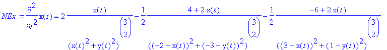
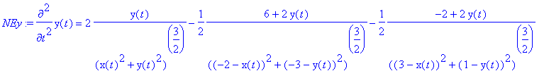
The superposition principle tells us that the x - and y -components of the position vector are calculated by the integration of the respective Newton equation components. However, as is evident from the expressions for Ex and Ey , the motions in x and y are coupled.

We choose particles of unit mass and unit charge:

> m:=1; q:=1;

> NEx:=m*diff(x(t),t$2)=q*Ex(x(t),y(t));

> NEy:=m*diff(y(t),t$2)=q*Ey(x(t),y(t));

To specify the initial conditions we have to make a choice of radius and pick the number of trajectories to emerge from the vicinity of the positve charge. We pick a larger value of r0 than before, so that the acceleration due to the positive charge at the center does not completely dominate the motion. In other words: we do not wish the probe particle to pick up too much speed.

> r0:=0.5; t:='t':

> IC:=i->[x(0)=r0*cos(phi(i)),D(x)(0)=0,y(0)=r0*sin(phi(i)),D(y)(0)=0];

> sol:=dsolve({NEx,NEy,op(IC(1))},{x(t),y(t)},numeric,output=listprocedure);

> xt:=subs(sol,x(t)): yt:=subs(sol,y(t)):

We check that the numerical integration works, i.e., it gives numerical answers for the position as a function of time:

> xt(1);

We pick a time interval at which the trajectory will be recorded:

> dt:=0.1;

> r02:=r0^2:

> Rt:=[[r0*cos(phi(1)),r0*sin(phi(1))]]: for it from 1 to 100 do: t:=it*dt; Xt:=xt(t); Yt:=yt(t); Rt:=[op(Rt),[Xt,Yt]]: if Xt^2+Yt^2> 200 then break fi; od:

One trajectory worked, so we complete the loop:

> for j from 2 to Nt do:

> t:='t': sol:=dsolve({NEx,NEy,op(IC(j))},{x(t),y(t)},numeric,output=listprocedure):

> xt:=subs(sol,x(t)): yt:=subs(sol,y(t)):

> Rt:=[op(Rt),[r0*cos(phi(j)),r0*sin(phi(j))]]: for it from 1 to 100 do: ti:=it*dt; Xt:=xt(ti); Yt:=yt(ti); Rt:=[op(Rt),[Xt,Yt]]: if Xt^2+Yt^2> 200 then break fi; od: od:

> PL4:=plot(Rt,style=point,symbol=cross,color=green,view=[-6..6,-6..6],axes=boxed,scaling=constrained): display(PL1,PL4);

We observe that the attraction to the negative charges located at P1 and P2 influences appreciably only those trajectories that pass by closely. We may want to observe what happens to probe particles that are started at rest from a larger distance.

Also note that the trajectories for the cases where the fixed negative charges are almost hit by the probe particle may be calculated inaccurately.

> t:='t':

> r0:=1.5;

> IC:=i->[x(0)=r0*cos(phi(i)),D(x)(0)=0,y(0)=r0*sin(phi(i)),D(y)(0)=0];

> sol:=dsolve({NEx,NEy,op(IC(1))},{x(t),y(t)},numeric,output=listprocedure);

> xt:=subs(sol,x(t)): yt:=subs(sol,y(t)):

> xt(1);

We pick a time interval at which the trajectory will be recorded:

> dt:=0.1;

> r02:=r0^2:

> Rt:=[[r0*cos(phi(1)),r0*sin(phi(1))]]: for it from 1 to 100 do: ti:=it*dt; Xt:=xt(ti); Yt:=yt(ti); Rt:=[op(Rt),[Xt,Yt]]: if Xt^2+Yt^2> 200 then break fi; od:

> for j from 2 to Nt do:

> t:='t': sol:=dsolve({NEx,NEy,op(IC(j))},{x(t),y(t)},numeric,output=listprocedure):

> xt:=subs(sol,x(t)): yt:=subs(sol,y(t)):

> Rt:=[op(Rt),[r0*cos(phi(j)),r0*sin(phi(j))]]: for it from 1 to 100 do: t:=it*dt; Xt:=xt(t); Yt:=yt(t); Rt:=[op(Rt),[Xt,Yt]]: if Xt^2+Yt^2> 200 then break fi; od: od:

> PL4:=plot(Rt,style=point,symbol=cross,color=green,view=[-6..6,-6..6],axes=boxed,scaling=constrained): display(PL1,PL4);

We observe that for the particles which were started at a large distance away from the central charge the deflection by the two other charges are more noticeable. This is so as the particles have a lower kinetic energy as they encounter the negative fixed charges. They were started further away from the central charge, and therefore have a lower potential energy at t =0. As a result the majority of particles no longer appear to follow simple almost straight lines as was the case before.

Exercise 1:

Pick your own locations of three charges in the plane in addition to a strong central charge. Graph the potential, construct the field lines, and graph real charged-particle trajectories that start in the vicinity of the central charge. Make observations about the field lines as well as the trajectories.

Exercise 2:

Pick locations and strengths for a few static charges in the plane. Solve the Newton equation for probe charge trajectories starting at the left of the chosen contourplot window for the potential moving to the right. Vary the initial speed for the probe charges and comment on the observed trajectories. Repeat the analysis for probe charges of the opposite sign.

>