Quantum Computation and Quantum Information
Michael A. Nielsen, Isaac L. Chuang (Cambridge, 2000) ISBN 0 521 63235 8.
Maple implementation by Marko Horbatsch (Computational Physics using Maple; www.yorku.ca/marko) August 2002, modified Oct. 2003.
We implement the matrix representation for a few quantum logic gates, such as the conditional NOT, derive the swap, the Hadamard gate, the formation of entangled states and work through quantum teleportation.
| > | restart; |
| > | with(LinearAlgebra): |
We introduce a basis for a 2-qubit; the first is the control qubit, the second is the target qubit; they form an entangled state.
| > | s00:=Vector([1,0,0,0]); |
| > | s01:=Vector([0,1,0,0]): s10:=Vector([0,0,1,0]): s11:=Vector([0,0,0,1]): |
The conditional NOT gate of quantum computing leaves the control qubit as is, and adds the target and control bit in binary logic.
The following picture is taken from the text (Fig. 1.6):

![[Maple OLE 2.0 Object]](images/Qubit2.gif)
| > | U_cnot:=Matrix([[1,0,0,0],[0,1,0,0],[0,0,0,1],[0,0,1,0]]); |
| > | U_cnot . s00, U_cnot . s01, U_cnot . s10, U_cnot . s11; |
In order to verify the truthtable we need to compare two vectors. Maple's evalb is unreliable when it performs this comparison, the results change between versions. Thus we define our own procedure Evalb , which compares equations with Vector objects on both sides component by component:
| > | Evalb:=proc(VectorEqn::`=`) local L,R,dL,dR,i,res; L:=lhs(VectorEqn): R:=rhs(VectorEqn): |
| > | if type(L,Vector) and type(R,Vector) then dL:=op(1,L): dR:=op(1,R): if dR<>dL then RETURN(false) fi: |
| > | for i from 1 to dL do: res:=simplify(R[i]-L[i]): if res <> 0 then RETURN(false): fi: od: RETURN(true): |
| > | else evalb(VectorEqn): fi: end: |
Now apply it to our case:
| > | Evalb(U_cnot . s00 = s00); |
![]()
| > | Evalb(U_cnot . s01 = s01); |
![]()
| > | Evalb(U_cnot . s10 = s11); |
![]()
| > | Evalb(U_cnot . s11 = s10); |
![]()
We see that: when the control qubit (qubit 1) is zero, the target qubit is left unchanged, and when qubit 1 has value 1, then qubit 2 is flipped. This represents the conditional NOT. We have verified eq. (1.18).
Now one should verify using binary arithmetic that given the notation |A> and |B> for the control and target qubits that |B> goes into |A+B>.
| > | true and true, true and false, false and true, false and false; |
![]()
| > | true or true, true or false, false or true, false or false; |
![]()
This does not implement 0 + 0 = 0, 0 + 1 = 1 + 0 = 1, 1 + 1 = 0 !
But the XOR between boolean states does do the desired thing:
| > | true xor true, true xor false, false xor true, false xor false; |
![]()
Note: the linearity of matrix multiplication will guarantee that we only need to know the action for the transformation matrix on basis states. The expansion coefficients, which measure how much probability amplitude we have in either state factor out linearly.
Now let us understand how three conditional NOTs can form a swap, as explained in eq. (1.20), and figure 1.7.
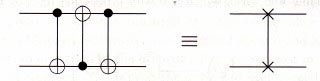
![[Maple OLE 2.0 Object]](images/Qubit12.gif)
The prescription is to apply the conditional NOT gate twice as done above, but sandwiched in-between is one action of the gate reversed (where the target quibit controls the control qubit). First we have to find the matrix that will do that! Let's make a guess, and transpose the two non-zero 2-by-2 blocks that form U_cnot.
| > | U_rcnot:=Matrix([[0,1,0,0],[1,0,0,0],[0,0,1,0],[0,0,0,1]]); |
Let us verify the action of this transformation matrix:
| > | U_rcnot . s00, U_rcnot . s01, U_rcnot . s10, U_rcnot . s11; |
The question is: did we flip qubit 1 depending on qubit 2 being 0 or 1, and leave qubit 2 alone? Let's compare:
| > | s00, s01, s10, s11; |
What did we generate above?
| > | s01,s00,s10,s11; |

We kept qubit 1, while flipping qubit 2 when qubit 1 was |0>, rather than |1>. So this matrix was not what we wanted! How should we find the right matrix?
We want the outcomes:
|00> -> |00> , |10> -> |10> , |01> -> |11> , |11> -> |01>
We could set up a system of equations to determine the matrix (cannon approach to swat a fly). It makes more sense to write the source and target spinors side-by-side, and to determine the required coupling coefficient.
| > | s00,s00; |
The first row better have a 1 in its first entry (and be [1,0,0,0] ?)
| > | s10,s10; |
The third row better be [0,0,1,0], or at least have a 1 in the third entry.
| > | s01,s11; |
The second row (producing the action for |01>) should have a zero in the second column. The fourth row has to produce the 1 in the fourth column, while it acts on s01. So it needs a 1 in the second column.
| > | s11,s01; |
| > | U_try:=Matrix([[1,0,0,0],[0,0,0,1],[0,0,1,0],[0,1,0,0]]); |
| > | Evalb(U_try . s00 = s00); |
![]()
| > | Evalb(U_try . s01 = s11); |
![]()
| > | Evalb(U_try . s10 = s10); |
![]()
| > | Evalb(U_try . s11 = s01); |
![]()
OK, so apparently this does what we want! Now let's compute the action of swapping circuit:
| > | U_swap:=U_cnot . U_try . U_cnot; |
Indeed, this is the matrix listed on page XXV for the swap! What does the swap do?
| > | U_swap . s00,s00; |

| > | U_swap . s01, s10; |

| > | U_swap . s10, s01; |

| > | U_swap . s11, s11; |

Note that swapping is not the same as inverting both qubits. This would agree on the 2nd and 3rd case, but not the first and fourth.
Exercise1:
Find the matrix which inverts both qubits. Construct this matrix carefully by comparing source and target qubit spinors.
Solution to Exercise 1
| > | s00,s11; |
first column in fourth row needs a 1.
| > | s10,s01; |
third column in second row needs a 1
| > | s01,s10; |
second column in third row needs a 1
| > | s11,s00; |
fourth column in first row needs a 1
| > | U_inv:=Matrix([[0,0,0,1],[0,0,1,0],[0,1,0,0],[1,0,0,0]]); |
| > | U_inv . s00, s11; |
| > | U_inv . s10, s01; |
| > | U_inv . s01, s10; |

| > | U_inv . s11 , s00; |

| > |
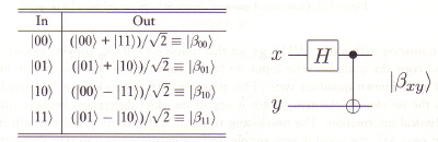
The Hadamard gate matrix can be used to create so-called Bell states, or entangled states as explained in Fig. 1.12.
First one applies the 2-by-2 Hadamard gate to the control qubit, and then carries out a conditional NOT.
Entangled states are such 2-qubit states which are not factorizable as a product of single-qubit states.
Here is Fig. 1.12:
![[Maple OLE 2.0 Object]](images/Qubit40.gif)
| > | H2:=Matrix([[1,1],[1,-1]])/sqrt(2); |
In order to be able to work this out with our 2-qubit states, we need to embed the Hadamard matrix so that it will act on qubit 1 in the 2-qubit state in spinor representation. We want to mix the components associated with qubit 1 irrespective of what's going on in qubit2.
| > | s00,s10,s01,s11; |
| > | s00+s10; |
| > | s01+s11; |
We really have to construct the Hadamard matrix acting on qubit 1. Naive embedding doesn't work! What is it that we want?
H2 |00> = s2 (|00> + |10>) , H2 |10> = s2 (|00> - |10>) , H2 |01> = s2 (|01> + |11>) , H2 |11> = s2 (|01> - |11>) ; where s2 = 1/sqrt(2).
| > | s00, s00 + s10; |
| > | s01, s01 + s11; |
| > | s10, s00 - s10; |
| > | s11, s01 - s11; |
| > | sq2:=1/sqrt(2): |
| > | H2q1:=Matrix([[sq2,0,sq2,0],[0,sq2,0,sq2],[sq2,0,-sq2,0],[0,sq2,0,-sq2]]); |
| > | H2q1 . s00, s00 + s10; |
| > | H2q1 . s01, s01 + s11; |
| > | H2q1 . s10, s00 - s10; |
| > | H2q1 . s11, s01 - s11; |
OK, so it worked. Now we can complete the action, by following up on H2q1 by a cNOT gate, which is not decomposable, and therefore leads to an entangled 2-qubit state:
| > | B:=U_cnot . H2q1; |
Figure 1.12 can now be verified:
| > | B . s00 , s00 + s11; |
| > | B . s01 , s01 + s10; |
| > | B . s10 , s00 - s11; |
| > | B . s11 , s01 - s10; |
Exercise 2:
Construct the matrix for the Hadamard gate for qubit2, and then compute the matrix H4 which performs the Hadamard gate on both qubits.
Solution to Exercise 2
First, we have to state the goal:
| > | s00, s00 + s01; |
| > | s10, s10 + s11; |
| > | s01, s00 - s01; |
| > | s11, s10 - s11; |
Therefore:
| > | H2q2:=Matrix([[sq2,sq2,0,0],[sq2,-sq2,0,0],[0,0,sq2,sq2],[0,0,sq2,-sq2]]); |
Let's verify:
| > | H2q2 . s00, s00 + s01; |
| > | H2q2 . s10, s10 + s11; |
| > | H2q2 . s01, s00 - s01; |
| > | H2q2 . s11, s10 - s11; |
OK, now take the matrix product:
| > | 2* H2q1 . H2q2; |
We multiplied by 2 to have a clear view of the matrix. Without the factor of 2 we have computed the Hadamard matrix W4, which represents the application of a Hadamard gate to both qubits. It is obtained as an outer product of two Hadamard gates W2 for each qubit (the order did not matter). An outer product represents a factorizable operation. The important thing to produce the Bell states was to apply U_cnot, the conditional NOT gate, which is represented by a matrix that cannot be factorized into two matrices acting on qubit 1 and qubit 2 separately.
| > |
Quantum Teleportation
According to Fig. 1.13 an entangled pair shared between two remote communication partners A and B (A=Alice, B=Bob) can be used to transfer a quantum state from one end to the other by means of a few gates, and a classical communication channel by which the outcome of a measurement done at A can be transmitted to B. The unknown state |psi> = a|0> + b|1> is being transferred from A to B, i.e., while B will be able to reconstruct it, A will wind up with a destroyed state. This has to be so to be compliant with the no-cloning theorem, which does not permit to duplicate quantum states.
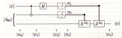
![[Maple OLE 2.0 Object]](images/Qubit69.gif)
The main idea: A has 2 lines, a control qubit line on which it stores originally the state |psi>, and a target qubit line on which is encoded one half of the entangled 2-qubit state. B has one line on which it has encoded the other qubit of the entangled state. The entire system, therefore, is a 3-qubit state, and the objective is to transfer the information from qubit 1 (Alice) to qubit 3 (Bob).
Alice will apply a cNOT followed by a Hadamard gate on q1, and then measure probabilities on q1 and q2. These probabilities will be transmitted classically to Bob, who will then know which gate to apply to q3, such that it will contain |psi> as originally stored on q1. Our aim is to calculate the evolution of the states.
To be able to apply the cNOT and Hadamard gates we need to set up A's 2-qubit state. The overall state is a product of |psi> = a|0> + b |1>, and
1/sqrt(2) (|00> + |11>). There are eight (2^3) possible basis states.
| > | s000:=Vector([1,0,0,0,0,0,0,0]): s001:=Vector([0,1,0,0,0,0,0,0]): s010:=Vector([0,0,1,0,0,0,0,0]): s011:=Vector([0,0,0,1,0,0,0,0]): s100:=Vector([0,0,0,0,1,0,0,0]): s101:=Vector([0,0,0,0,0,1,0,0]): s110:=Vector([0,0,0,0,0,0,1,0]): s111:=Vector([0,0,0,0,0,0,0,1]): |
Now we need to define the cNOT gate for q1 and q2. We need an 8-by-8 matrix that serves as an embedding of the 4-by-4 cNOT gate, and which ignores the state of q3.
| > | s000,s001; |
Both these states are to be left unchanged.
| > | #UcNOT:=Matrix([[1,0,],[0,1,],[],[],[],[],[],[]]): |
Also the next two should be left as is:
| > | s010,s011; |
| > | #UcNOT:=Matrix([[1,0,0,0,],[0,1,0,0,],[0,0,1,0,],[0,0,0,1,],[],[],[],[]]): |
| > | s100,s110,s101,s111; |
In the above two pairs: the first spinor is to be transformed into the second.
| > | #UcNOT:=Matrix([[1,0,0,0,0,0,0,0],[0,1,0,0,0,0,0,0],[0,0,1,0,0,0,0,0],[0,0,0,1,0,0,0,0],[0,0,0,0,0,0,],[0,0,0,0,0,0,],[0,0,0,0,1,0,0,0],[0,0,0,0,0,1,0,0]]): |
and finally, the remaining pair of pairs:
| > | s110,s100,s111,s101; |
| > | UcNOT:=Matrix([[1,0,0,0,0,0,0,0],[0,1,0,0,0,0,0,0],[0,0,1,0,0,0,0,0],[0,0,0,1,0,0,0,0],[0,0,0,0,0,0,1,0],[0,0,0,0,0,0,0,1],[0,0,0,0,1,0,0,0],[0,0,0,0,0,1,0,0]]); |
Check it out:
| > | Evalb(UcNOT . s000 = s000) ,Evalb(UcNOT . s001= s001); |
![]()
| > | Evalb(UcNOT . s010 = s010) ,Evalb(UcNOT . s011 = s011); |
![]()
| > | Evalb(UcNOT . s100 = s110) , Evalb(UcNOT . s101 = s111); |
![]()
| > | Evalb(UcNOT . s110 = s100) , Evalb(UcNOT . s111 = s101); |
![]()
Now construct the Hadamard gate matrix representation for q1.
| > | sq2; |
![]()
| > | s000, s000 + s100, s001, s001 + s101; |
We will start with a matrix filled by zeroes, and will replace the non-zero entries according to the requirements.
| > | Hq1:=Matrix(8,8): |
| > | Hq1[1,1]:=sq2: Hq1[5,1]:=sq2: Hq1[2,2]:=sq2: Hq1[6,2]:=sq2: |
| > | s010, s010 + s110, s011, s011 + s111; |
| > | Hq1[3,3]:=sq2: Hq1[7,3]:=sq2: Hq1[4,4]:=sq2: Hq1[8,4]:=sq2: |
| > | s100, s000 - s100 , s101, s001 - s101; |
| > | Hq1[1,5]:=sq2: Hq1[5,5]:=-sq2: Hq1[2,6]:=sq2: Hq1[6,6]:=-sq2: |
| > | s110, s010 - s110 , s111, s011 - s111; |
| > | Hq1[3,7]:=sq2: Hq1[7,7]:=-sq2: Hq1[4,8]:=sq2: Hq1[8,8]:=-sq2: |
| > | Hq1; |
| > | Determinant(Hq1); |
![]()
Let's check it out... we copy the lines used for the matrix construction, and turn them into equations to be checked:
| > | Evalb(sqrt(2)*Hq1 . s000 = s000 + s100), Evalb(sqrt(2)*Hq1 . s001 = s001 + s101); |
![]()
| > | Evalb(sqrt(2)*Hq1 . s010 = s010 + s110), Evalb(sqrt(2)*Hq1 . s011 = s011 + s111); |
![]()
| > | Evalb(sqrt(2)*Hq1 . s100 = s000 - s100) , Evalb(sqrt(2)*Hq1 . s101 = s001 - s101); |
![]()
| > | Evalb(sqrt(2)*Hq1 . s110 = s010 - s110) , Evalb(sqrt(2)*Hq1 . s111 = s011 - s111); |
![]()
Now we are able to put the teleportation gate together: Equation 1.29 states the initial |psi>.
| > | psi:=sq2*(a*(s000 + s011) + b*(s100 + s111)); |

| > | psi:=simplify(psi); |
| > | psi1:= UcNOT . psi; |
| > | psi2:= Hq1 . psi1; |
What is the significance of psi2 as compared to the initial psi, i.e., what was the effect of applying the gates? Somehow, the information (values of a,b) got transferred all over the place. Note, Alice never knew what her amplitudes a and b were, and the claim is, that if she measures the probability content of q1 and q2, and transmits it classically to Bob, then Bob can infer what simple gate to apply in order to re-surrect the superposition a|0> + b|1> in 'his' qubit, i.e., in q3 (without knowing the values of a,b). How can we find out whether this indeed works?
The claim is, that if Alice measures a |00>, then Bob simply has a|0> + b|1> in q3. For Alice observing |01>, he gets b|0> + a|1>, for Alice measuring |10> he gets a|0> - b|1>, and when she sees |11>, he obtains -b|0> + a|1>. This means that upon receiving information from Alice on the classical channel as to what she measured on q1/q2, Bob can apply a corresponding transformation (in the latter three cases) in order to rotate the state into a|0> + b|1>, thus receiving psi.
How do we obtain the collapse of psi2 to a single-qubit wavefunction, i.e., what do we do to simulate Alice's measurement?
It is a projection onto the 2-qubit state that should do the trick. Two degrees of freedom would be contracted away, with a remaining two-spinor wavefunction.
One way to convince oneself, is to realize which superposition the state psi2 represents:
| > | phi2:=simplify((a*s000+b*s001) + (a*s011+b*s010) + (a*s100-b*s101) + (a*s111-b*s110)); |
| > | Evalb(phi2=2*psi2); |
![]()
The four states above are grouped in such a way that they correspond to Alice's four possible measurement outcomes, namely |00> (in which case qubit 3 is in the original state of q1), |01>, |10>, and |11>.
This calculation then carries out the matrix representation of eqs. 1.28 to 1.36.
Classical computing with qubits: Toffoli gate
The idea is to demonstrate the a classical NAND gate can be implemented on a quantum computer. This will be very inefficient, but is interesting from a fundamental point of view: a quantum computer, in principle, can be built to simulate a classical computer.
![[Maple OLE 2.0 Object]](images/Qubit96.gif)

A 3-qubit gate which allows to simulate NAND gates, is a reversible gate which has 3 inputs and 3 outputs, whereby the first two qubits act as control qubits.
| > | T:=Matrix(8,8): T[1,1]:=1: T[2,2]:=1: T[3,3]:=1: T[4,4]:=1: T[5,5]:=1: T[6,6]:=1: T[7,8]:=1: T[8,7]:=1: |
| > | Determinant(T); |
![]()
| > | Evalb(T . s111 = s110); |
![]()
One can verify the truth table given in Fig. 1.14. A NAND gate can be obtained by using the first two qubits as input, setting the third input to 1, and using the q3 output as the result. Another application is by using it as a FANOUT, i.e., a bit readout gate (by setting q1=1, q3=0 on input, and obtaining q3=q2=a for q2=a input.
Exercise 3:
Go through the truth table of the Toffoli gate, and verify the NAND gate behaviour described above.
| > |