Uncertainty principle for angular momentum states
How can we demonstrate the minimum uncertainty for orbital angular momentum states?
We wish to demonstrate that for operators satisfying [A,B]=C the minimum uncertainty dA*dB = <C>*h_/2;
[h_ stands for h-bar].
For A=L_x, B=L_y, C=i h_ L_z. We would need to look at, e.g., psi an eigenstate of L_z, so the right-hand side is sharp, and we know psi.
Given that psi we can calculate:
a) the time evolution of the expectation values;
b) the average value of L_x, and L_y, and their uncertainties;
c) check the above relationship for the uncertainties.
We need the spherical harmonics (eigenstates of L^2 and L_z).
The angular parts are spherical harmonics.:
> restart; with(orthopoly);
![]()
> Plm:=proc(theta,l::nonnegint,m::integer) local x,y,f;
> x:=cos(theta);
> if m>0 then f:=subs(y=x,diff(P(l,y),y$m));
> else f:=subs(y=x,P(l,y)); fi;
> (-1)^m*sin(theta)^m*f; end:
> Plm(theta,3,2);
![]()
For the spherical harmonics we don't need the Plm's with negative argument.
> Y:=proc(theta,phi,l::nonnegint,m::integer) local m1;
> m1:=abs(m); if m1>l then RETURN("|m} has to be <= l for Y_lm"); fi;
> exp(I*m*phi)*Plm(theta,l,m1)*(-1)^m*sqrt((2*l+1)*(l-m1)!/(4*Pi*(l+m1)!)); end:
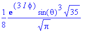
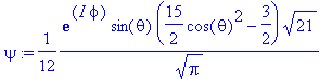
> Y(theta,phi,3,0);
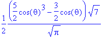
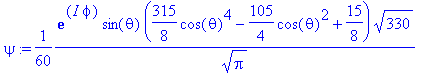
> Y(theta,phi,3,1);
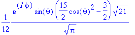
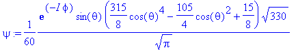
> Y(theta,phi,3,2);
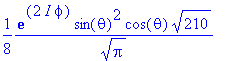
> Y(theta,phi,3,3);
> No:=(l,m)->int(int(evalc(Y(theta,phi,l,m)*conjugate(Y(theta,phi,l,m))),phi=0..2*Pi)*sin(theta),theta=0..Pi);
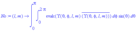
> No(1,0);
![]()
> No(1,1);
![]()
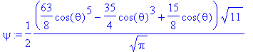
> No(3,2);
![]()
> Y(theta,phi,0,0);
![]()
Uncertainty in L_x and L_y for an L_z eigenstate
Suppose psi is the state with 5 units of h_ (h-bar) measured for L_z. Let us also specify that it is the state with L^2 eigenvalue of 5*(5+1) h_^2.
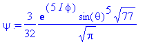
> psi:=Y(theta,phi,5,5);
What are the expectation values of L_x and L_y?
To answer this question we need to either express L_x and L_y in spherical polar coordinates, and calculate the expectation in these coordinates, or we switch the eigenfunction over to Cartesian coordinates.
> LzOP:=f->-I*h_*simplify(diff(f,phi));
![]()
> LzOP(psi)/psi;
> simplify(LzOP(psi)/psi,trig);
![]()
We have verified that the state psi has eigenvalue 5 h-bar for the L_z operator. Let us define the operators for L_x and L_y:
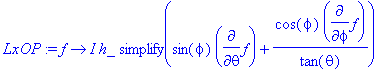
> LxOP:=f->I*h_*simplify(sin(phi)*diff(f,theta)+cos(phi)/tan(theta)*diff(f,phi));
> LyOP:=f->I*h_*simplify(-cos(phi)*diff(f,theta)+sin(phi)/tan(theta)*diff(f,phi));
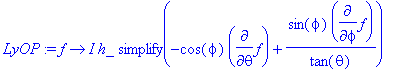
These definitions follow from a straightforward application of the transformation from Cartesian to spherical polar coordinates of L_x, L_y, and L_z.
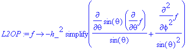
We can also define the angular momentum squared operator in spherical polar coordinates:
> L2OP:=f->-h_^2*simplify(diff(sin(theta)*diff(f,theta),theta)/sin(theta)+diff(f,phi$2)/sin(theta)^2);
> L2OP(psi)/psi;
> simplify(%);
![]()
This is consistent with 5*(5+1)*h_^2. We can verify that the result from L2OP is consistent with the result calculated from Lx^2+Ly^2+Lz^2:
> L2OPlong:=f->LxOP(LxOP(f))+LyOP(LyOP(f))+LzOP(LzOP(f));
![]()
> L2OPlong(psi)/psi;

![]()
![]()
> simplify(%);
![]()
Let us verify that the state psi is not an eigenstate of L_x, or L_y:
> LxOP(psi)/psi;
> simplify(%);
![]()
Clearly this is a function of theta and phi! Therefore L_x |psi> is not proportional to |psi>. A similar result is obtained for L_y.
What are the average values (expectation values) for L_x and L_y while the particle is in state |psi> ?
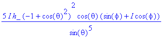
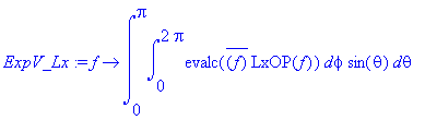
> ExpV_Lx:=f->int(int(evalc(conjugate(f)*LxOP(f)),phi=0..2*Pi)*sin(theta),theta=0..Pi);
> ExpV_Lx(psi);
![]()
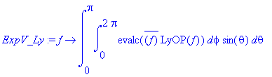
> ExpV_Ly:=f->int(int(evalc(conjugate(f)*LyOP(f)),phi=0..2*Pi)*sin(theta),theta=0..Pi);
> ExpV_Ly(psi);
![]()
On average the particle has zero value in the components of L_x and L_y.
Just to confirm our previous result for L_z obtained via the eigenvalue:
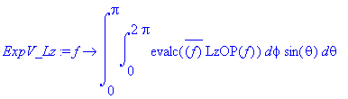
> ExpV_Lz:=f->int(int(evalc(conjugate(f)*LzOP(f)),phi=0..2*Pi)*sin(theta),theta=0..Pi);
> ExpV_Lz(psi);
![]()
Now we can define the uncertainties (via their squares):
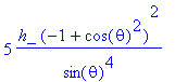
> dLxsq:=f->int(int(evalc(conjugate(LxOP(f))*LxOP(f)),phi=0..2*Pi)*sin(theta),theta=0..Pi)-ExpV_Lx(f)^2;

> dA:=sqrt(dLxsq(psi));
![]()
> dLysq:=f->int(int(evalc(conjugate(LyOP(f))*LyOP(f)),phi=0..2*Pi)*sin(theta),theta=0..Pi)-ExpV_Ly(f)^2;

> dB:=sqrt(dLysq(psi));
![]()
> dA*dB;
![]()
This shows that the state psi has the minimum uncertainty allowed under the uncertainty principle which follows from the commutation relation [L_x, L_y] = I h_ L_z.
The RHS of the uncertainty relation dA*dB >= h_/2 |<C>| where C = I*h_*L_z equals the LHS for our particular eigenstate. We notice that the state psi (5 units of angular momentum in the z-direction) has an avaerage value of 0 for each of the components that cannot be measured exactly with an uncertainty of sqrt(10)/2 h_
> evalf(sqrt(10)/2);
![]()
What are the uncertainties for a state whose L_z eigenvalue is not maximal (i.e., for which M is less than L )?
Before we proceed with the calculations for the L=5 multiplet, let us verify that the uncertainty (deviation) is zero for the L_z component, as the system is in an L_z eigenstate:
> dLzsq:=f->int(int(evalc(conjugate(LzOP(f))*LzOP(f)),phi=0..2*Pi)*sin(theta),theta=0..Pi)-ExpV_Lz(f)^2;
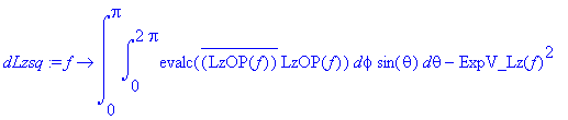
> dLzsq(psi);
![]()
Indeed we find that for an eigenstate the uncertainty in the measurement is zero.
We proceed with the check of the uncertainty relation for eigenstates of L_z with eigenvalues M < L :
> psi:=Y(theta,phi,5,4);
> dA:=sqrt(dLxsq(psi));
![]()
> evalf(%);
![]()
> dB:=sqrt(dLysq(psi));
![]()
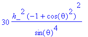
> dA*dB;
![]()
This is to be compared with the right-hand side of:
> h_/2*4*h_;
![]()
We conclude that the uncertainty is much larger than for maximal L_z eigenstate! In fact, the uncertainty principle is now realized not with the minimal uncertainty, but the LHS grew larger, while the RHS was smaller than for the maximal L_z eigenstate! Can this behaviour be generalized?
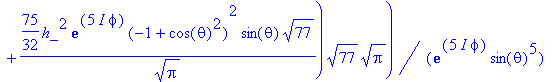
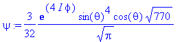
> psi:=Y(theta,phi,5,3);
> sqrt(dLxsq(psi)),sqrt(dLysq(psi));
![]()
> evalf(%);
![]()
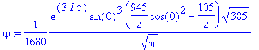
> psi:=Y(theta,phi,5,2);
> sqrt(dLxsq(psi)),sqrt(dLysq(psi));
![]()
> evalf(%);
![]()
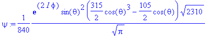
> psi:=Y(theta,phi,5,1);
> sqrt(dLxsq(psi)),sqrt(dLysq(psi));
![]()
> evalf(%);
![]()
> psi:=Y(theta,phi,5,0);
> sqrt(dLxsq(psi)),sqrt(dLysq(psi));
![]()
> evalf(%);
![]()
> psi:=Y(theta,phi,5,-1);
> sqrt(dLxsq(psi)),sqrt(dLysq(psi));
![]()
> evalf(%);
![]()
Indeed we do find that the product of the uncertainties for L_x and L_y grows with decreasing M , while the RHS of the uncertainty principle gets smaller (it vanishes for M =0 eigenstates of L_z). Remarkably, for the states with maximal z -projection (the two states with M = L and M =- L ) we find that they are minimum-uncertainty eigenstates of the angular momentum operators.
These observations are consistent with the diagram that shows the multiplet of angular momentum states displayed as vectors whose endpoints lie on a sphere of radius squared equal to L ( L +1) h_^2, with L_z component sharply defined as M h_, and undetermined L_x and L_y: the tip of the angular momentum vector lies on a circle that intersects the sphere at height z = M h_.
Why do the states with maximal z -projection have the smallest uncertainty in Lx and Ly? These are the states where most of the angular momentum vector resides in the z -component which is known exactly. On the other hand in the case of M =0 we have the largest uncertainty, as all of the angular momentum is in the x - and y - components. Ironically, the uncertainty principle would allow us the smallest (zero) uncertainty for these states in principle. This result from the generalized uncertainty principle is required so that it remains valid for the L = M =0 eigenstates (whose eigenfunction is a constant). For these particular states all three components L_x, L_y, and L_z are determined to have zero eigenvalue, i.e., are known exactly. Note that this represents the only case when [L_x, L_y] = i h_ L_z can be satisfied, and still L_x and L_y are compatible for these eigenstates.
Exercise 1:
Repeat the above calculations for orbital angular momentum states of a different L-value. What happens in the case of L = M =0?
Verification of the angular momentum commutation relations
We can use the operators to verify some commutation relations by acting on an unspecified function of the angles theta and phi. Watch out for the order in which the operators act on the function:
> CR1:=LxOP(LyOP(f(theta,phi)))-LyOP(LxOP(f(theta,phi)))=I*h_*LzOP(f(theta,phi)):
Note how evalb does not carry out a simplification: one has to be careful while using it.
> evalb(CR1);
![]()
> evalb(simplify(CR1));
![]()
> simplify(lhs(CR1));
![]()
The amount of required simplifications is formidable.
> CR2:=L2OP(LxOP(f(theta,phi)))-LxOP(L2OP(f(theta,phi))):
> simplify(CR2);
![]()
>
Visualization of orbital angular momentum states
We can use sphereplot to visualize the spherical harmonics. We look at the density, and keep in mind that Maple follows the mathematics and not the physics convention for naming the angles in spherical polar coordinates. For us physicists theta is the polar and phi the azimuthal angle.
> with(plots):
Warning, the name changecoords has been redefined
> psi:=Y(theta,phi,3,1);
> rho:=evalc(conjugate(psi)*psi);

>
sphereplot(rho,phi=0..2*Pi,theta=0..Pi,style=patchcontour,color=phi,axes=boxed,numpoints=3000,scaling=constrained,style=wireframe,thickness=2);
![[Maple Plot]](images/Uncertainty70.gif)
Exercise 2:
Look at the visualizations of other angular momentum eigenstates. Rotate the diagram to observe the projections onto particular planes (e.g., the x - z plane), and compare with textbook diagrams. What is the meaning of these diagrams in the context of the probabilistic interpretation of wavefunctions?
Can we graph the diagram for the visualization of the angular momentum vector? The plottools package allows us to graph spheres and cones.
We pick units in which h_ equals unity. To visualize the knowledge available for the angular momentum vector in an L >0 eigenstate we use a cone: the height of the cone is used to indicate the sharply known z -projection. The indeterminacy of the x - and y - components is combined with the knowledge that the average value of either of these components is zero, and that the deviations (uncertainties) are the same in both components. This makes it obvious that the Lx and Ly values are determined to be somewhere on a circle of a known radius (determined by the uncertainty). Unlike in classical mechanics where the complete angular momentum vector is known precisely (and conserved for motion in central potentials) our knowledge of this vector in quantum mechanics is incomplete. The mantle of the cone visualizes the possible locations of the L vector in the sense of a bundle of vectors: given a measurement of L^2 and L_z (after which we are in an |LM> eigenstate) we only know that Lx and Ly have values such that the L vector lies on the mantle of the cone. Of course, a measurement of either L_x or L_y would destroy the |LM> eigenstate (a subsequent remeasurement of L_z would lead to any of the allowed M -values). Therefore, this picture has to be taken with a grain of salt.
> L:=5;
![]()
> r:=sqrt(L*(L+1));
![]()
> with(plottools):
> s:=sphere([0,0,0],r,color=green):
> M:=4: R:=sqrt(r^2-M^2):
> c2a:=cone([0,0,0],R,M,color=red):
> M:=2: R:=sqrt(r^2-M^2):
> c2b:=cone([0,0,0],R,M,color=blue):
> M:=-3: R:=sqrt(r^2-M^2):
> c2c:=cone([0,0,0],R,M,color=magenta):
> C1:=display(s,style=wireframe,scaling=constrained,axes=boxed):
> C2a:=display(c2a,style=patchnogrid,scaling=constrained,axes=boxed):
> C2b:=display(c2b,style=patchnogrid,scaling=constrained,axes=boxed):
> C2c:=display(c2c,style=patchnogrid,scaling=constrained,axes=boxed):
> display([C1,C2a,C2b,C2c],labels=[x,y,z],orientation=[150,65]);
![[Maple Plot]](images/Uncertainty73.gif)
Exercise 3:
Look at the graphical representation for different values of L and M .
Matrix representation of the angular momentum algebra
We can ask the following question: given that the spherical harmonics are realizations of the angular momentum algebra for L , M eigenstates in the coordinate representation ( L , M being integers), are there other representations as well?
The problem is to construct matrices that represent the L_x, L_y, L_z observables; find representations in which L_z and L^2 are diagonal, while the other two are represented by non-diagonal, i.e., non-commuting matrices. A systematic approach based on ladder operators can be developed (commut2.mws).
It turns out that two linear combinations of L_x and L_y play the role of raising and lowering operators. Let us verify this in the coordinate representation:
> phi1:=Y(theta,phi,5,3);
> simplify(LxOP(phi1)+I*LyOP(phi1));

> simplify(%/Y(theta,phi,5,4));
![]()
> evalc(%);
![]()
> simplify(%,trig);
![]()
Clearly the action of L_x+I*L_y on the state |5,3> led to a state propotional to |5,4>. The factor can be checked to be consistent with the analytical result:
> L:='L': M:='M': subs(L=5,M=3,h_*sqrt((L-M)*(L+M+1)));
![]()
This result agrees (apart from a minus sign) with the ratio found above.
Let us check that L_x-I*L_y lowers the magnetic quantum number:
> simplify(LxOP(phi1)-I*LyOP(phi1));

> simplify(%/Y(theta,phi,5,2));
![]()
> evalc(%);
![]()
> simplify(%,trig);
![]()
> L:='L': M:='M': subs(L=5,M=3,h_*sqrt((L+M)*(L-M+1)));
![]()
As for the L(+) operator we find that the lowering operator L(-) produces the lowered normalized state up to a well-defined factor.
We have verified by example that the combinations L(+) := L_x + i L_y and (L-) := L_x - i L_y act as ladder operators which allow us to step through the eigenstates in a given ( LM )-multiplet. One can look at the action of the products L(+) L(-) and L(-)L(+) to establish the allowed range of M -values.
Our objective is now to generalize on the basis of the ideas behind orbital angular momentum. We are looking for a realization of the angular momentum algebra with substantially fewer degrees of freedom: instead of the orbital angular momentum operators which act of functions of theta and phi (polar and azimuthal angle) we are interested in operators that act on so-called spinors. The spinors are in the simplest case column vectors of numbers of size N (such as the [1,0] and [0,1] basis vectors representing spin alignment and counter-alignment with a given axis), and the operators are given as N -by- N matrices that mix the components of spinors while acting on them.
We define the matrices that represent the components of an J=1/2 angular momentum operator.
> with(linalg):
Warning, the protected names norm and trace have been redefined and unprotected
> S_x:=matrix([[0,h_/2],[h_/2,0]]);
![S_x := matrix([[0, 1/2*h_], [1/2*h_, 0]])](images/Uncertainty85.gif)
> S_y:=matrix([[0,-I/2*h_],[I/2*h_,0]]);
![S_y := matrix([[0, -1/2*I*h_], [1/2*I*h_, 0]])](images/Uncertainty86.gif)
> S_z:=matrix([[h_/2,0],[0,-h_/2]]);
![S_z := matrix([[1/2*h_, 0], [0, -1/2*h_]])](images/Uncertainty87.gif)
> S2:=evalm(S_x &* S_x + S_y &* S_y + S_z &* S_z);
![S2 := matrix([[3/4*h_^2, 0], [0, 3/4*h_^2]])](images/Uncertainty88.gif)
> evalm(S_x &* S_y - S_y &* S_x);
![matrix([[1/2*I*h_^2, 0], [0, -1/2*I*h_^2]])](images/Uncertainty89.gif)
Clearly this agrees with I*h_ S_z.
The eigenvectors of S_z and S^2 are the spinor solutions [1,0] and [0,1].
Exercise 4:
Verify the commutation relations for the other permutations of [ x , y , z ], i.e., demonstrate that S_x, S_y, and S_z satisfy the angular momentum algebra.
Exercise 5:
Verify the angular momentum algebra for higher spinor representations (S=1, and S=3/2 matrices are defined below). Calculate the eigenvectors of S_z. Comment on the eigenvalues of S_z and S^2, and on the uncertainty principle.
> S1_x:=evalm(h_/sqrt(2)*matrix([[0,1,0],[1,0,1],[0,1,0]]));
![S1_x := matrix([[0, 1/2*h_*sqrt(2), 0], [1/2*h_*sqr...](images/Uncertainty90.gif)
> S1_y:=evalm(h_/sqrt(2)*matrix([[0,-I,0],[I,0,-I],[0,I,0]]));
![S1_y := matrix([[0, -1/2*I*h_*sqrt(2), 0], [1/2*I*h...](images/Uncertainty91.gif)
> S1_z:=evalm(h_*matrix([[1,0,0],[0,0,0],[0,0,-1]]));
![S1_z := matrix([[h_, 0, 0], [0, 0, 0], [0, 0, -h_]]...](images/Uncertainty92.gif)
> S3o2_x:=evalm(h_/2*matrix([[0,sqrt(3),0,0],[sqrt(3),0,2,0],[0,2,0,sqrt(3)],[0,0,sqrt(3),0]]));
![S3o2_x := matrix([[0, 1/2*h_*sqrt(3), 0, 0], [1/2*h...](images/Uncertainty93.gif)
> S3o2_y:=evalm(h_/2*matrix([[0,-I*sqrt(3),0,0],[I*sqrt(3),0,-2*I,0],[0,2,0,-I*sqrt(3)],[0,0,I*sqrt(3),0]]));
![S3o2_y := matrix([[0, -1/2*I*h_*sqrt(3), 0, 0], [1/...](images/Uncertainty94.gif)
> S3o2_x:=evalm(h_/2*matrix([[3,0,0,0],[0,1,0,0],[0,0,-1,0],[0,0,0,-3]]));
![S3o2_x := matrix([[3/2*h_, 0, 0, 0], [0, 1/2*h_, 0,...](images/Uncertainty95.gif)
>