Wavepackets in quantum mechanics

We look at solutions to the free-particle Schroedinger wave equation in one spatial dimension. The first step is to look at exact solutions to the equation for fixed momentum, i.e., for sharp energy. These plane-wave solutions are completely delocalized in space. Then we form superpositions from these states which have the property of being localized in space, and having a spread in momentum (i.e., free-particle energy). These solutions can be imagined to represent an ensemble of particles with a spread of momenta around an average value, i.e., to represent a beam of particles. The dispersion of such wavepackets in space with time is demonstrated; it can be explained due to the presence of faster and slower components in the ensemble.

The one-dimensional time-dependent Schroedinger wave equation (TDSE) for free particles is given as (eventually we choose units where hbar= m =1, we use h_ for hbar):

> restart;

> TDSE:=I*h_*diff(psi(x,t),t)=-h_^2/(2*m)*diff(psi(x,t),x$2);

The LHS of the TDSE can be interpreted as the energy operator acting on the wavefunction psi( x , t ), while the RHS represents the kinetic energy operator acting on psi( x , t ). This wave equation is different from the one known in classical electromagnetism: it represents waves of massive particles that obey the non-relativistic energy-momentum relationship (dispersion relation). The kinetic energy operator was formed on the basis of where the momentum operator is given as . Our first task is to demonstrate the form of the plane-wave solutions (the unfamiliar reader should look up the solution to the relativistic wave equation for electromagnetic waves in a first-year physics text before proceeding).

The wave equation denoted as TDSE is obviously separable in position and momentum: the solution should be given as a product of a time-dependent and a position-dependent factors. If we denote by E the energy of the particle, and by p its momentum value (a number, not to be confused with p-operator used above) we have the classical relationship for the free particle . Keeping in mind that the LHS of the TDSE represents the energy operator ( ) we are looking for a solution where the time-dependent factor when acted upon by the LHS produces the energy as a factor, while on the RHS we want the two derivatives with respect to x to do the same with the position-dependent factor. The only choice (apart from an overall multiplicative normalization factor) is:

> phi_p:=exp(-I/h_*p^2/(2*m)*t)*exp(I/h_*p*x);

We substitute

> subs(psi(x,t)=phi_p,TDSE);

and divide out the solution to observe that the answer is correct for any value of p :

> simplify(%/phi_p);

We have meaningful solutions for any real-valued p . For each energy E there are two solutions:

one which is right-travelling ( p >0), and one which is left-travelling ( p <0).

The wavefunctions phi_p are labeled therefore by their momentum value, indicating that we have found an infinite family of solutions. We think of the momentum value as being fixed for the particle. The interpretation of phi_p is that it represents a probability amplitude. The squared magnitude gives the probability to find the particle at some location in space x at a given time t .

> evalc(abs(phi_p)^2);

This, of course, is confusing. The result for the probability to find the particle at ( x , t ) is independent of position (at any time t ). Moreover, since the summation over all allowed positions involves an integral over the entire x -axis, there is a serious problem: we cannot find a normalization constant such that the sum over all probabilities remains finite. This represents a subtle problem that is associated with the infinite volume of space. In the real world this should not be a problem, and we can impose a finite volume (if worst comes to worst, the volume of the universe). For any finite volume the plane-wave solutions can be normalized such that the probabilistic interpretation is salvaged, but there is a price to pay: the freedom to choose any real-valued momentum (or energy) for the free particle will be sacrificed, as the boundary conditions (periodicity at the edges of the volume) will impose a volume-dependent discreteness of allowed momentum (energy) values.

For the sake of our discussion it will be advantageous at first to ignore this problem, and deal with solutions defined on the entire x -axis. We sacrifice the interpretation of the solution for the freedom to choose any energy value, and to use the simple unnormalized solutions phi_p. These solutions represent a complete basis set. Any function defined on the real axis that is a potential candidate for solving (satisfying) the TDSE can be expanded in this basis. For the sake of understanding the basis functions we look at the graphs of them, i.e., of their real and imaginary parts. Picking out the real (or imaginary) part can be done by hand, but one has to take into consideration both factors.

> Wr:=unapply(evalc(Re(phi_p)),p);

> Wi:=unapply(evalc(Im(phi_p)),p);

> h_:=1; m:=1;

> with(plots):

Let us observe the evolution of the real and imaginary parts of the plane wave for the case of p =1/2. We generate a sequence of snapshots in time, and graph over a fixed position range:

> PLf:=s->plot([subs(t=s,Wr(0.5)),subs(t=s,Wi(0.5))],x=-10..10,color=[red,blue]):

> PLs:=seq(PLf(it*0.2),it=0..50):

> display(PLs,insequence=true);

As expected, the real and imaginary parts of the plane wave remain in phase. The crests (and zeroes) travel with a speed that depends on the chosen momentum. The reader can verify this by choosing different values of p . For the case chosen of p =1/2 and t _fin = 10 units the phase of the wave traveled a distance of

Dx = 0.5 p t _fin

Therefore the phase velocity is only one half of what one might have expected naively. It is the result of the definition of the phase velocity as . We have for the wavenumber (in our units h_=1, i.e., k = p ), and the circular frequency is related to the energy as (in our units: ). Thus, we have for the phase velocity of a Schroedinger matter wave: .

It is important to realize that contrary to electromagnetic waves in vacuum (where all plane waves move with the velocity of light) the matter waves propagate with phase velocities that differ in magnitude for different momentum values. However, one does know that electromagnetic waves in a medium (when the Maxwell equations are coupled to an ionic plasma) follow a different dispersion relation which results in a slowdown compared to propagation in vacuum, and dispersion of wavepackets (for an elementary discussion see Richard W. Robinett: Quantum Mechanics , Oxford Unversity Press 1997, chapter 2).

Wavepackets

Clearly the phase velocity can not be the physically important quantity. Also, the complete delocalization of the plane waves appears to make them inappropriate for the description of a localized bunch of particles. Nevertheless, we will observe shortly that a superposition (linear combination) of plane waves can describe a localized wave. We begin by superimposing just a few plane waves, and graphing the result.

In fact, when choosing the superposition we will have the freedom to admix waves of certain momenta with pre-determined mixing coefficients. It is this momentum profile which we are free to choose that will lead to physically understandable propagation properties. Let us do the simplest-possible thing: we choose a window of a few discrete momentum values with plane waves at these momenta superimposed with equal mixing coefficients.

For the average momentum, the spread, and the number of waves we choose:

> p_avg:=1; Dp:=1/2; Np:=5;

The chosen discrete momentum values:

> p_d:=i->p_avg+Dp*(i-(Np+1)/2)/Np;

> seq(p_d(i),i=1..Np);

We choose real mixing coefficients, and can therefore superimpose the real and imaginary parts of the plane waves separately to form the real and imaginary parts of the wavepacket:

> WPr:=add(Wr(p_d(i)),i=1..Np):

> WPi:=add(Wi(p_d(i)),i=1..Np):

We proceed as before to obtain an animation of the time evolution, except that we add a graph of the magnitude squared (scaled down to fit on the same graph):

> PLf:=s->plot([subs(t=s,WPr),subs(t=s,WPi),0.3*(subs(t=s,WPr)^2+subs(t=s,WPi)^2)],x=-15..15,color=[red,blue,green]):

> PLs:=seq(PLf(it*0.1),it=0..50):

> display(PLs,insequence=true);

The magic seems to work:

1) We have obtained a localized object that can move.

2) The object moves at the expexted speed [5 distance units in 5 units of time for an average momentum of 1 unit]

Several questions remain, which should be explored by the reader (using modifications to the lines above):

1) What happens for narrower/wider momentum distributions (variation of Dp )?

2) Check the travel distance for different average momenta.

3) Does the wavepacket preserve its shape (unlikely due to the momentum spread)?

4) What happens at larger distances x ? Can the problem be ameliorated by choosing finer momentum discretizations (more superimposed plane-wave components)?

5) What are the signatures of a larger momentum spread? What can one say about the structures in the oscillations ahead of the centre, and behind it?

Gaussian wavepackets

Some of the concerns/questions raised above are resolved by considering a 'perfect' superposition: instead of summing over discrete momentum values we can integrate over the entire range of allowed momenta and weigh the plane waves with a momentum profile. A practical issue that arises is whether we can carry out the integral in closed form. For a Gaussian momentum profile, which is characterized by an average momentum and a width (standard deviation) the integral can be carried out, and the wavefunction (packet) can be calculated in the coordinate representation. The result is the so-called Gaussian wavepacket, which is localized in real space. It can be extended also to more than one spatial dimenstion.

The Gaussian (or other, e.g., Lorentzian) wavepacket maintains its momentum profile, which is consistent with free-particle propagation (no external forces). It spreads in position space due to the dispersion of the different plane-wave components (they move with different phase velocities). The wavepacket conspires to achieve this: the product of momentum and position uncertainties grows as a function of time (and does not violate Heisenberg's principle, as it involves an inequality). This dispersion is entirely consistent with classical dispersion. As long as one sticks to the ensemble interpretation of quantum mechanics there is no conceptual problem with this growth in uncertainty (delocalization due to dispersion). One does not attach meaning to the wavepacket as far as individual particles are concerned, one remains on the safe side by the statement that the Schroedinger wave equation describes an ensemble (and not individual particles). The ensemble, of course, can be realized sequentially (an example from a multiple-slit experiment: dots appear on a screen randomly one after the other, forming eventually an interference pattern that can be calculated by quantum mechanics).

> restart;

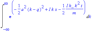
We proceed to carry out the integral which calculates psi( x , t ) from a plane wave superposition with a Gaussian profile centered at k = q . We need the following integral:

> Int(exp(-a^2/2*(k-q)^2+I*k*x-I*h_*k^2/(2*m)*t),k=-infinity..infinity);

Here the first argument in the exponential represents the superposition coefficient in which a controls the momentum spread (it has dimensions of length).

The argument in the exponential to be integrated is given as (the calculation tries to follow S. Fluegge: Practical QM I , Springer):

> arg:=-a^2/2*(k-q)^2+I*k*x-I*h_*k^2/(2*m)*t;

> factor(arg);

That doesn't do the job to complete the square.

> with(student):

> arg1:=completesquare(arg,k);

> assume(b>0);

> I1:=unapply(int(exp(-b^2*z^2),z=-infinity..infinity),b);

> I1(b);

This integral can be used (without checking the positivity of b ). We realize that a constant shift in z does not affect the result (the integration range remains the same). A stretching of the variable has the following effect:

> arg11:=op(1,arg1);

> k0:=solve(arg11,k);

For some reason solve repeats the solution. We will need to lift out one of them later, i.e., use k0[1] .

One can use the change of variables procedure that is part of the student package:

> assume(a>0,h_>0,t>0,m>0);

> changevar(k-k0[1]=y,Int(exp(arg1),k=-infinity..infinity),y);

> simplify(%): #Maple won't do it due to the shift of b into the complex plane

We use a cheat to reach the goal: our integral I1( b ) has been simplified under the assumption that b >0. It is, in fact, valid for Re( b )>0, implying a complex integration contour parallel to the real axis. Thus, we can carry out the k integration and need only to keep track of the x -dependent exponential factor.

> b0:=simplify(sqrt(arg11/(k-k0[1])^2));

> I1(b0);

> arg12:=op(2,arg1);

> arg12cs:=completesquare(arg12,x);

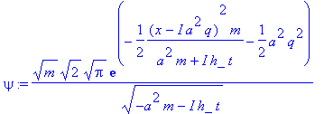
> psi:=I1(b0)*exp(arg12cs);

Note that psi still looks like a mess: it is not obvious what it describes, since x is not centered on a real value. The result appears to agree with the textbook calculation. The starnge form of psi is needed to accomplish the growing uncertainty in Dx Dp.

> factor(psi);

The density is easier to understand:

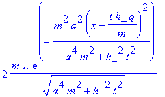
> rho:=evalc(simplify(abs(psi)^2));

> completesquare(rho,x);

Now it is evident that the density represents a Gaussian centered on the expected location: p =h_ q is the average momentum of the GWP, therefore the distance travelled by the position expectation value (starting at x =0 at t =0) is: s = v t = pt / m = t h_ q / m .

Let us check the normalization integral.

> int(rho,x=-infinity..infinity);

The normalization stays constant in time, but for a correct probabilistic interpretation we would need to adjust it by multiplying it with the factor sqrt(a/(2*Pi^(3/2))) .

For a graph we set a few obvious constants, and choose the average momentum, and the spread parameter:

> with(plots):

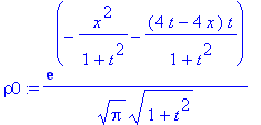
> rho0:=subs(h_=1,m=1,a=1,q=2,(a/(2*Pi^(3/2)))*rho);

> animate(rho0,x=-2..18,t=0..5,color=green,numpoints=200,frames=25);

> WPr:=evalc(Re(subs(h_=1,m=1,a=1,q=2,sqrt(a/(2*Pi^(3/2)))*psi))):

> WPi:=evalc(Im(subs(h_=1,m=1,a=1,q=2,sqrt(a/(2*Pi^(3/2)))*psi))):

> PLf:=s->plot([subs(t=s,WPr),subs(t=s,WPi),2*subs(t=s,rho0)],x=-5..20,color=[red,blue,green],title=cat("time= ",convert(s,string))):

> PLs:=[seq(PLf(it*0.2),it=0..25)]:

> display(PLs,insequence=true,view=[-5..20,-0.6..1.2]);

We observe the asymmetry of the oscillatory structure at the end of the propagation: the fast components ahead of the wavepacket are oscillating more quickly than the slow components left behind. This is not apparent at t=0. We explore this behaviour further by looking at the flux (current density).

We can calculate the flux of the wavepacket.

> j:=phi->(h_/(2*I*m))*(conjugate(phi)*diff(phi,x)-phi*diff(conjugate(phi),x));

> assume(q,real); assume(x,real);

> simplify(diff(psi,x)/psi);

What does this imply? The derivative of psi is proportional to psi and it is possible to factor out the density in j ( x , t ), as the same holds for the complex conjugate.

This is why it makes sense to simplify j ( x , t )/rho( x , t ). Exploration of the line below shows why the assumptions on q , x were needed.

> simplify(diff(conjugate(psi),x)/conjugate(psi));

> res:=simplify(j(psi)/rho); # This doesn't work without the assumptions on x and q!

According to classical flows (in hydrodynamics, or charge flows in electrodynamics) the current density can be interpreted as particle density times a local (position-dependent) velocity. Thus, we have calculated a position-dependent velocity field for the matter wavepacket. At time t =0 it is constant:

> simplify(subs(t=0,res));

At time zero the flux is given by a constant velocity times the density profile. At t =0 all particles described by the ensemble move with the same velocity irrespective of their location! At later times this changes as the result becomes x -dependent. The faster particles in the inital GWP ( k > q ) move further ahead, while the slower particles fall behind the average position. By how much the velocity profile changes depends on the width parameter a .

The velocity profile is real-valued:

> res:=simplify(evalc(res));

This is equivalent to Fluegge's eq. (17.12).

> res1:=simplify(subs(h_=1,m=1,a=1,q=2,res));

> P0:=plot(subs(t=0.1,res1),x=-5..10,color=black): P1:=plot(subs(t=1,res1),x=-5..10,color=red): P2:=plot(subs(t=2,res1),x=-5..10,color=blue): P3:=plot(subs(t=3,res1),x=-5..10,color=green): display(P0,P1,P2,P3);

These straight lines illustrate the dispersion: we can find the location of the average momentum value is space at a given time:

> l1:=simplify(subs(t=1,res1)); l2:=simplify(subs(t=2,res1)); l3:=simplify(subs(t=3,res1));

> solve(l1=2,x); solve(l2=2,x); solve(l3=2,x);

The velocity v = p / m is maintained at the center position of the WP at all times: for our choice of q =2 ( m =1) and times t =1,2,3 this happens at the locations x =2,4,6. Furthermore, it is evident that the velocity dispersion is linear!

The graphs illustrate that something dramatic happens to the velocity profile early on (0< t <1), and that it becomes less interesting later on.

> animate(res1,x=-5..10,t=0..5,frames=30,color=blue);

Note that despite of the fact that the WP moves forward with an appreciable velocity on average, and has a constant 'local velocity' at t =0, the Gaussian distribution of velocities at t =0 does imply the presence of some negative velocity components. A small part of the WP moves backwards. In the ensemble interpretation of the WP it means that there are some particles that move to the left. The velocity distribution alone, of course, does not reveal what fraction of particles described by the WP carries out this 'non-intuitive' motion.

If we had been more careful to normalize at t =0 we would be getting a conserved probability of unity, but the main point is that our WP maintains its normalization!

The animation of the WP motion performed further above doesn't show flux moving to the left. We can make it more evident by plotting the logarithm of the density (the natural logarithm calculates much faster since it simplifies).

> rho0l:=simplify(log(rho0)):

> animate(rho0l,x=-5..15,t=0..5,view=[-5..15,-10..0],frames=30,color=red,numpoints=200);

What is the interpretation of these results?

Initially there can be no correlation between the particle position and its momentum. The density at negative values of x is dominated by right-moving components. The simultaneous knowledge of a constant velocity profile ( v ( x , t )= j ( x , t )/rho( x , t )) and a momentum distribution prescribed by Fourier analysis (which is a consequence of localization of the GWP in coordinate space!) is puzzling, to say the least.

Eventually the dominating right-moving components move away from the x <0 region, and we can see the appearance of left-moving parts. These appear also to arrive from the x >0 region. Wherever the original density profile was 'squeezed' (curvature in psi), there was a large momentum uncertainty, which implies also noticable left-moving contributions in this case. The log-plot allows one to observe what is masked in the regular graph of the density.

>