F 2005: Classes will be held on Wednesdays 9:30-11:25 in Stong 304 (NOTE THE ROOM CHANGE! - Stong is the college opposite to Bethune). Students are expected to pre-read the notes. For the next class (Sept 21), please go over sections 2.1-2.6. This is review material, we will cover it quickly. If you would like me to spend time at the end on computing in Maple, please send me an e-mail.
Marking scheme: Four assignments and one final test on the last day of classes, each worth 20%.
Our final test (on Hamiltonian mechanics) will be held on Monday, Dec.12 2005, between 10 am and 4 pm (it should require no more than 2-3 hours).
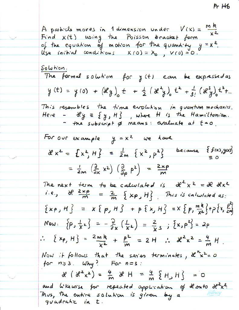
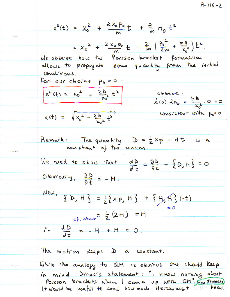
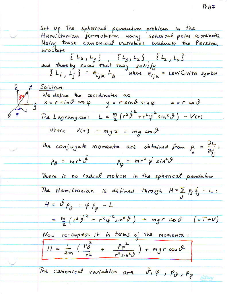
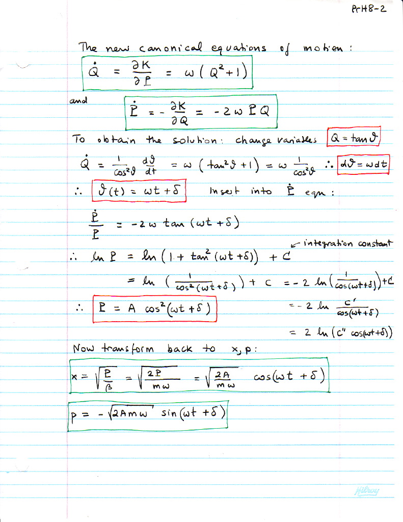
Notes for problems discussed in class. P1_page1; P1_page2; P2_page1; P2_page2; P3_page1; P3_page2;
The worksheets on dynamical systems that I used in the Dec. 16 class are part of the Computational Physics using Maple project, namely 8.2 and 8.3 there.
Fourth assignment: Pencil-and-paper work: Construct the Hamiltonian for a heavy, symmetrical top with one point fixed, and the top exposed to earth's gravitational field. Derive Hamilton's equations of motion, and compare them with Lagrange's equations given in Fetter-Walecka in chapter 31.
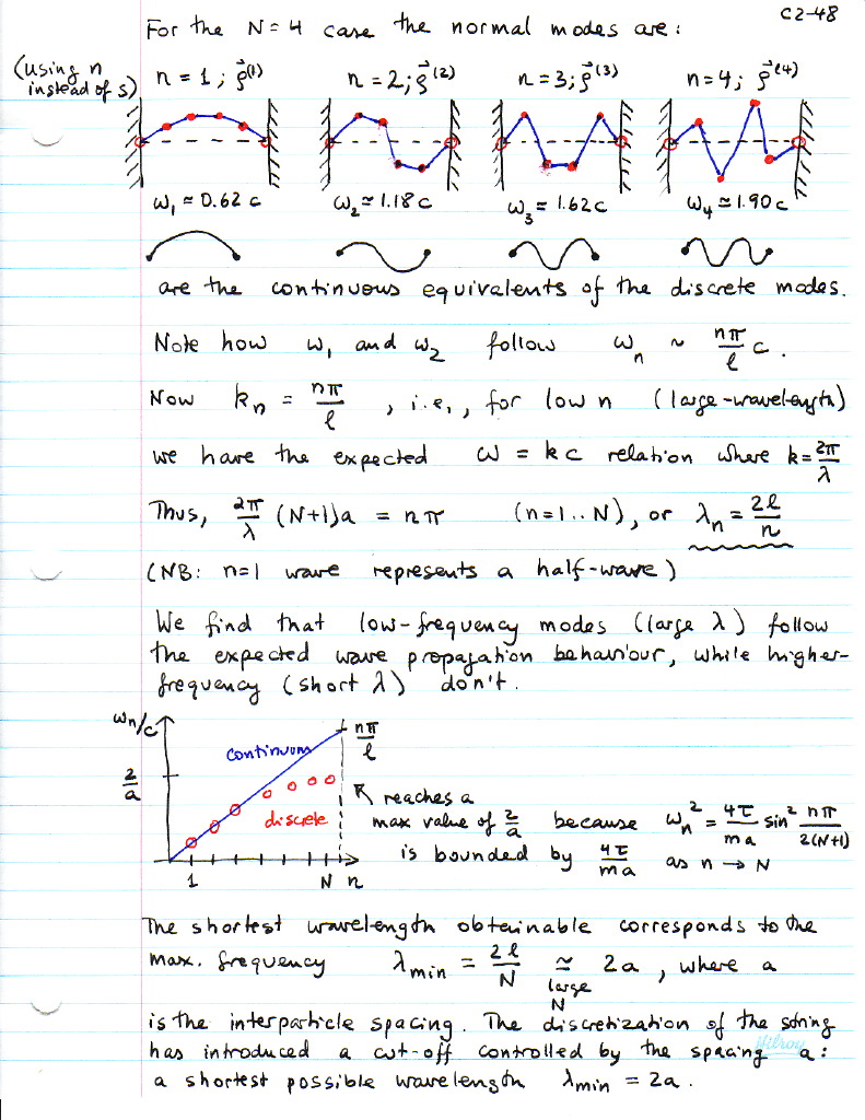
Third assignment: Use a computing environment of your choice to produce the graphs on page C2-48 for several values of N (start with the ones given on the page, then increase N, e.g., to N=10 and 20). Then repeat the procedure for periodic boundary conditions. Comment on the discrete vs continuous dispersion relation based on your results.
Second assignment (theoretical part): Derive the equations of motion for coupled planar pendula. Many undergrad texts do this with some approximations. We need the full equations, because in the practical part we will solve Lagrange's equations and will investigate the system for chaotic behaviour. Try the derivation of the Lagrangian on your own using the two angles with respect to the vertical as generalized coordinates. Do not linearize the pendulum. Assume masses m and M for the lower and upper mass, and the same arm length a for the upper and lower arm. The arms are assumed to be massless. Therefore, these are coupled mathematical pendula (moments of inertia is, e.g., m*a^2, i.e., we make the point mass approximation).
SOLUTION TO Assignment2 in Maple (numerical part): http://www.yorku.ca/marko/ComPhys/DblPendulum/DblPendulum.html
Second assignment (computational part): Write a program in a programming environment of your choice that contains a black box for solving ordinary differential equations (Maple, Mathematica, Matlab, etc.) to solve the problem of 2 planar coupled pendula and demonstrate by example the sensitivity to initial conditions. For Maple/Matlab you can find the code in my notes for PHYS 2030.
http://www.yorku.ca/marko/PHYS2030/Notes/Notes.html
For Maple a numerical solution example is shown on page 1.15 of the notes. For Matlab it is on page 1.19. In Fortran or C you could get yourselves a Runge-Kutta solver out of Numerical Recipes by W.P. Press et al.
SOLUTION TO Assignment1 in Maple: http://www.yorku.ca/marko/ComPhys/ClassicalScattering/ClassicalScattering.html
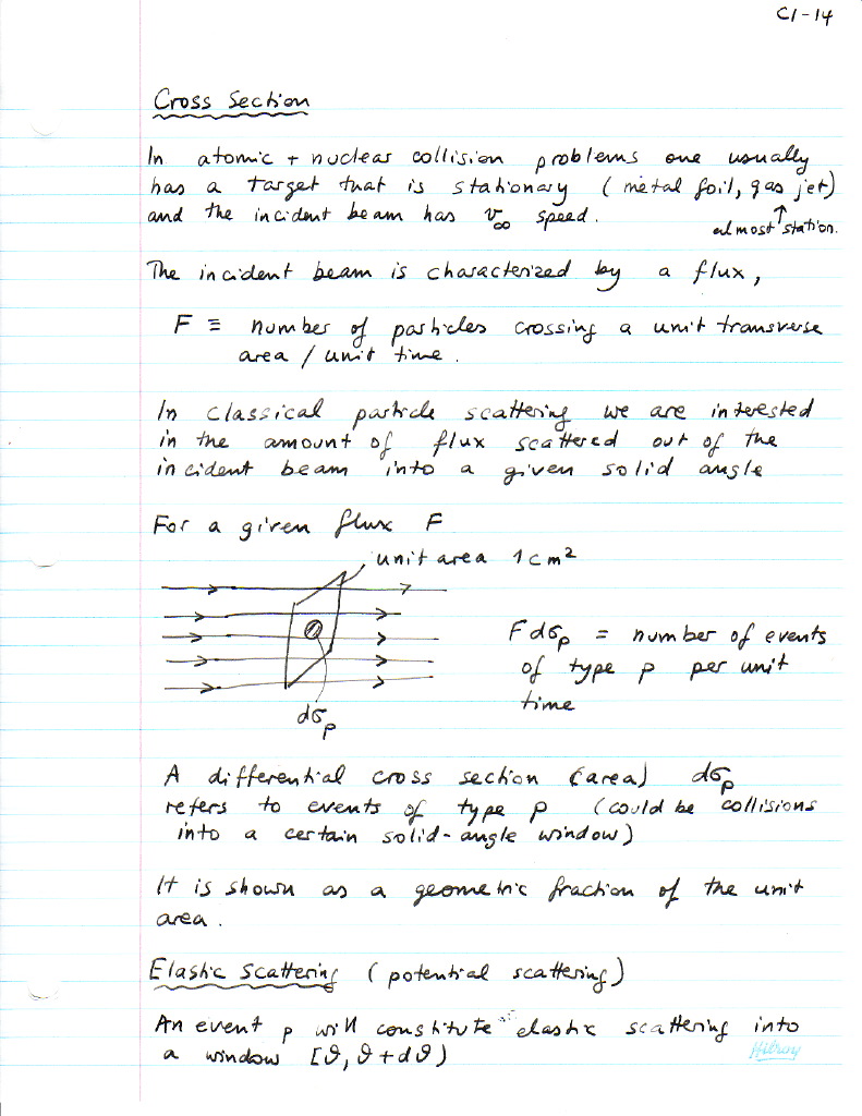
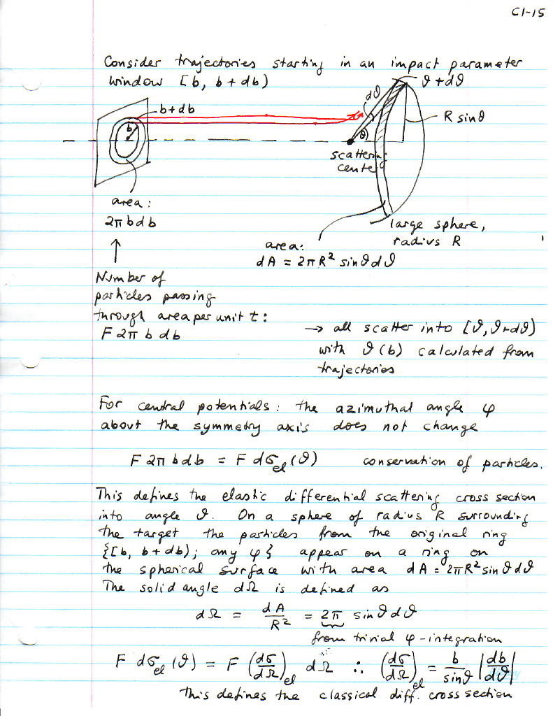
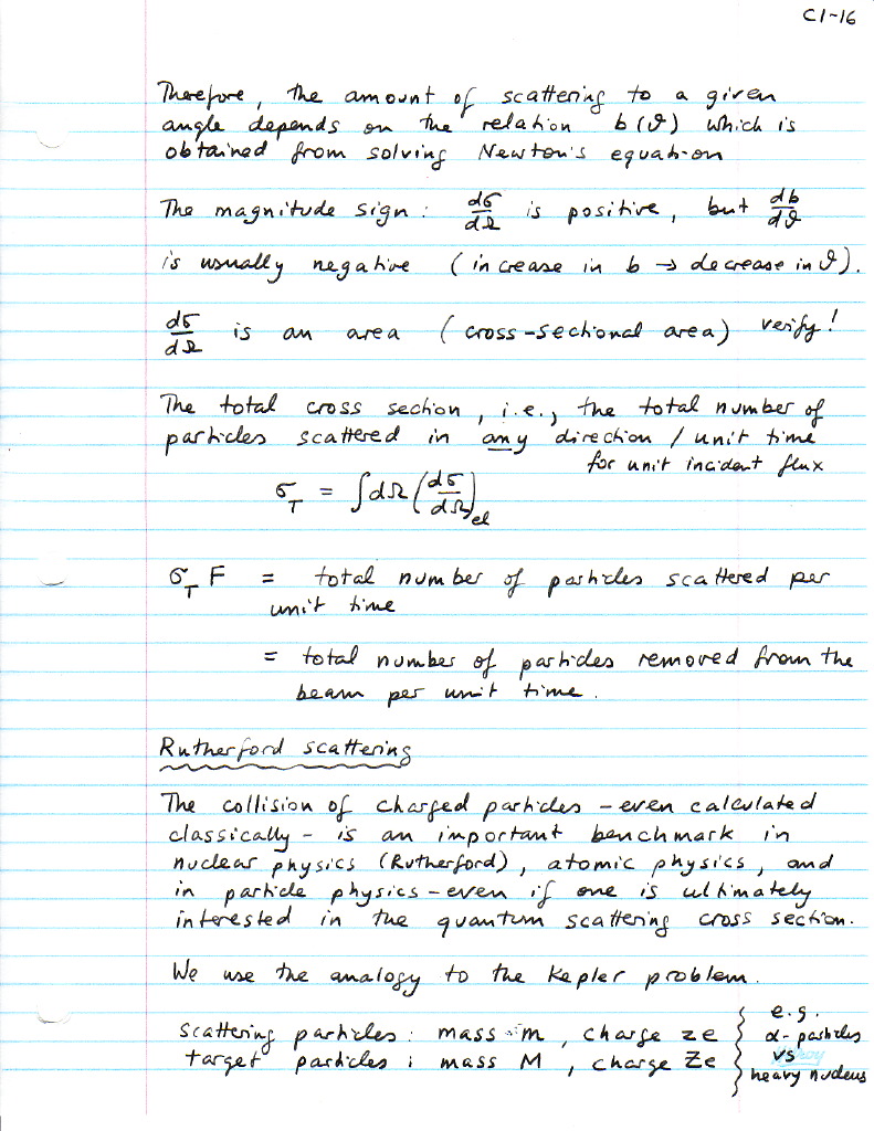
First assignment (due Sept 28): Investigate the b(theta) relationship and calculate the differential cross section numerically for a screened Rutherford (Bohr) potential. Make a choice of projectile/target charges and masses, use reasonable units (e.g., Bohr units in which e=m_e=1 (and also hbar=1)), and pick at least one scattering energy. In Bohr units a velocity v=1 (Bohr electron velocity in the 1s state) corresponds to a scattering energy of 25 keV for a proton. First test your code on the Rutherford case itself, for which the answers are given in the notes (and in most textbooks). Then multiply the Rutherford (Coulomb) potential by exp(-r/a), where a is of the order of the Bohr radius, calculate numerically a table of impact parameter b versus scattering angle theta, and then differentiate the relationship numerically to arrive at the differential cross section. Numerical differentiation with a central difference formula: f'(x) = [f(x+dx)-f(x-dx)]/(2*dx). Make sure you understand for which impact parameters the two cross sections (screened and unscreened) should agree.
One approach would be to use an integrator to solve Newton's law, which in Maple is provided in the following worksheet: Kepler.html; Kepler.mws;
Another, more elegant approach is to use Newton's law in once integrated form. Energy conservation allows to perform one integration. Fetter&Walecka in Eqs. (5.15, 5.16 a and b) show that a root search for the distance of closest approach needs to be combined with a numerical integral.
Course Synopsis
The course presents Lagrangian and Hamiltonian mechanics including canonical transformations and Hamilton-Jacobi theory. In the beginning (introduction and Lagrangian mechanics) it follows the text of A.L. Fetter and J.D. Walecka [1]. For phase-space methods, canonical transformations, and action-angle variables it relies on the text by I. Percival and D. Richards [2]. The final portions on the Hamilton-Jacobi theory are borrowed from L.D. Landau and E.M. Lifshits [3]. Problems are assigned mostly out of H. Goldstein (2nd or 3rd ed.) [4].
Ref # [1] QA 808.2 F47; [2] QA 614.8 P47; [3] QA 805 L283; [4] QA 805 G6.
For Goldstein,Poole,Safko (3rd ed.) an extensive error list (including our contributions) is available at 3d edition errors
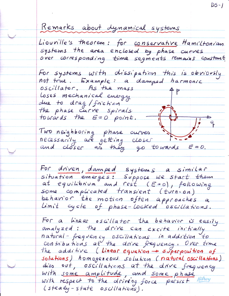
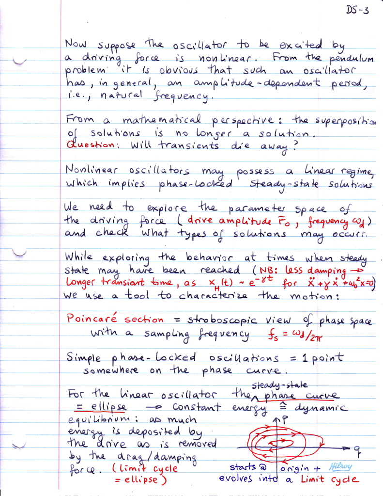
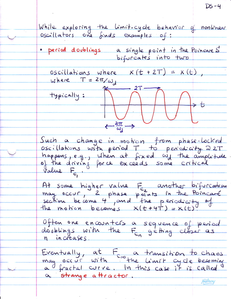
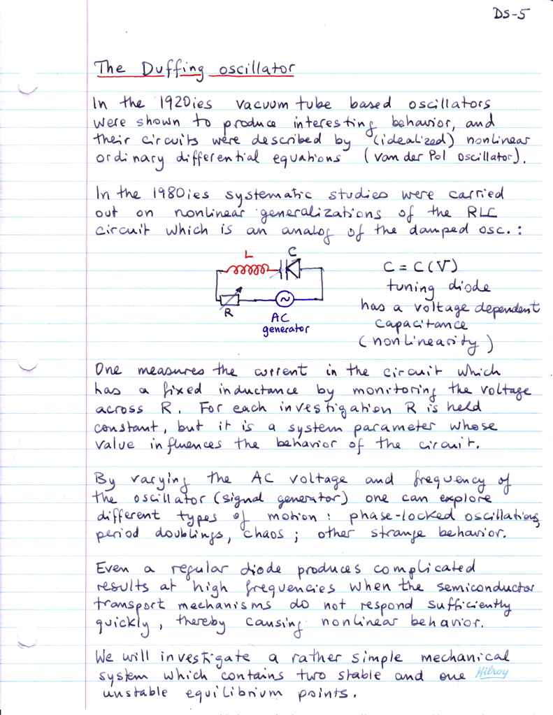
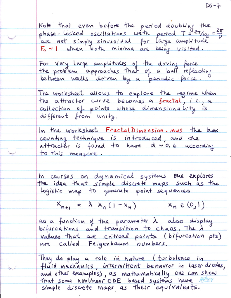
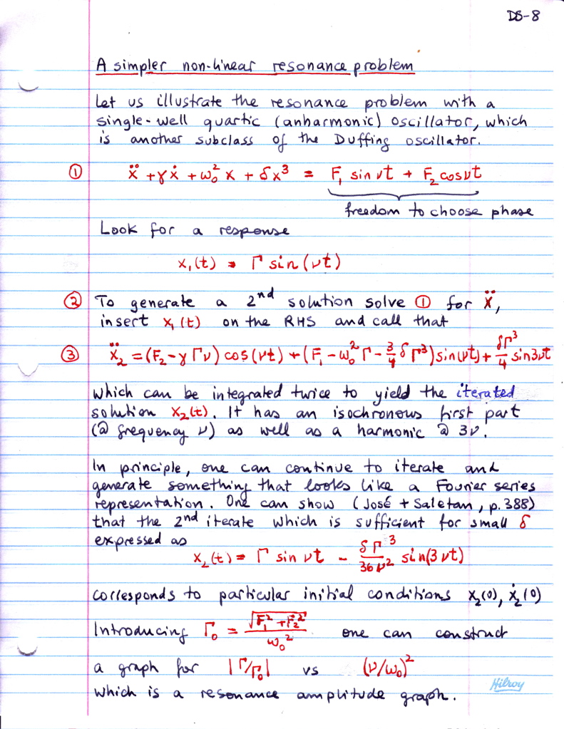
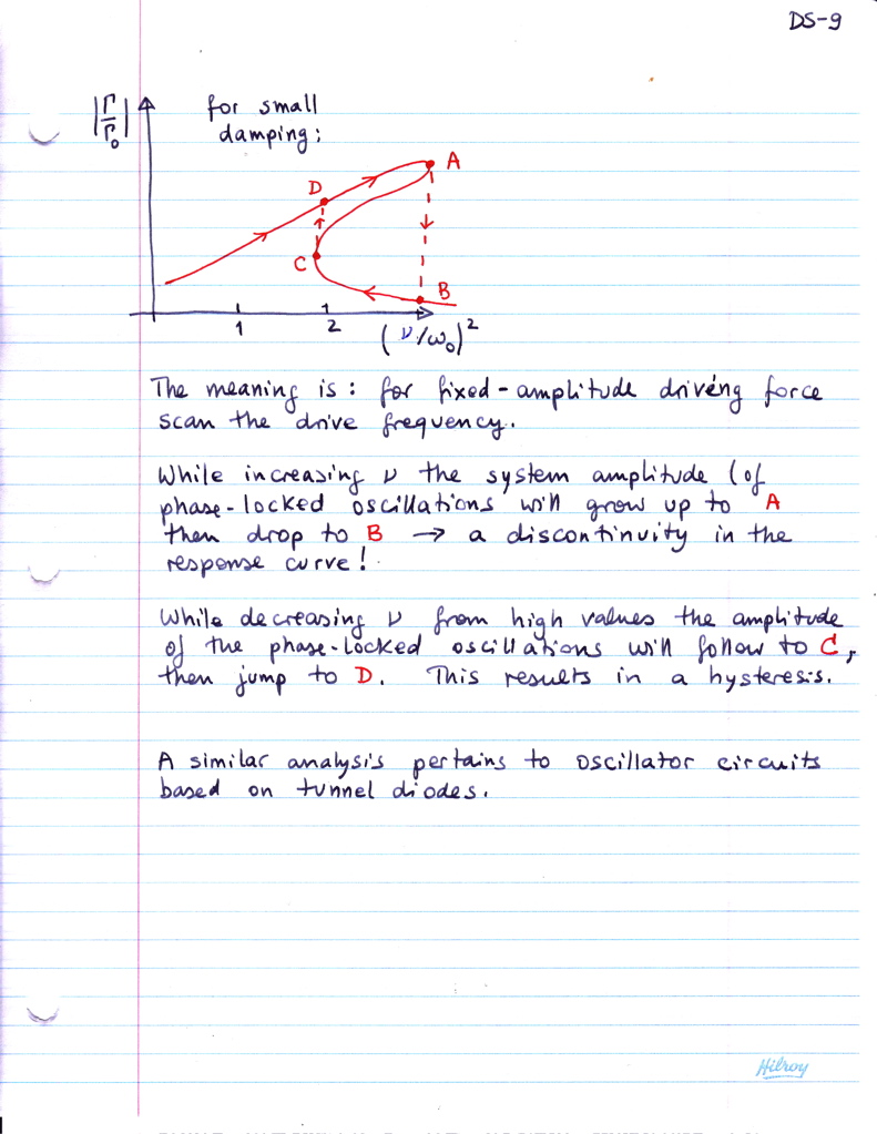
Lecture notes for dynamical systems, covered after phase space, Liouville theorem, before action angle variables (class of Nov. 16).
DS1 DS2 DS3 DS4 DS5 DS6 DS7 DS8 DS9
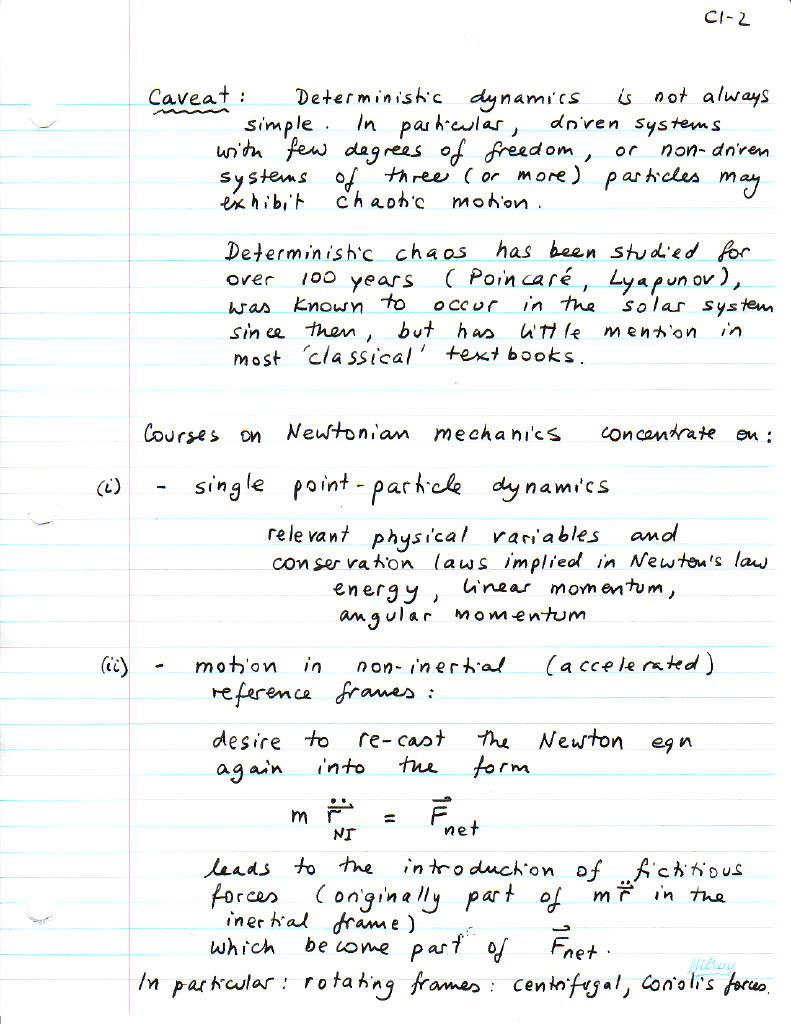
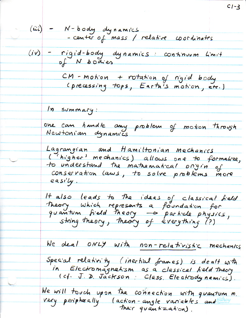
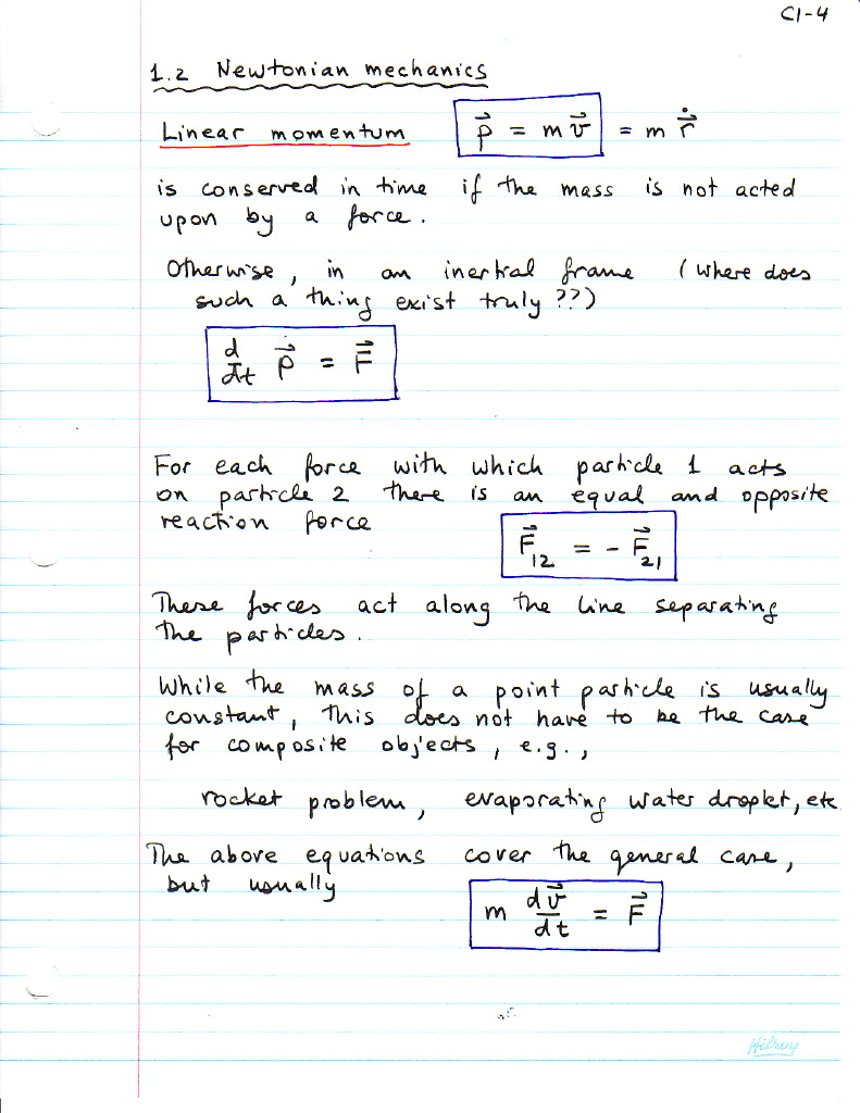
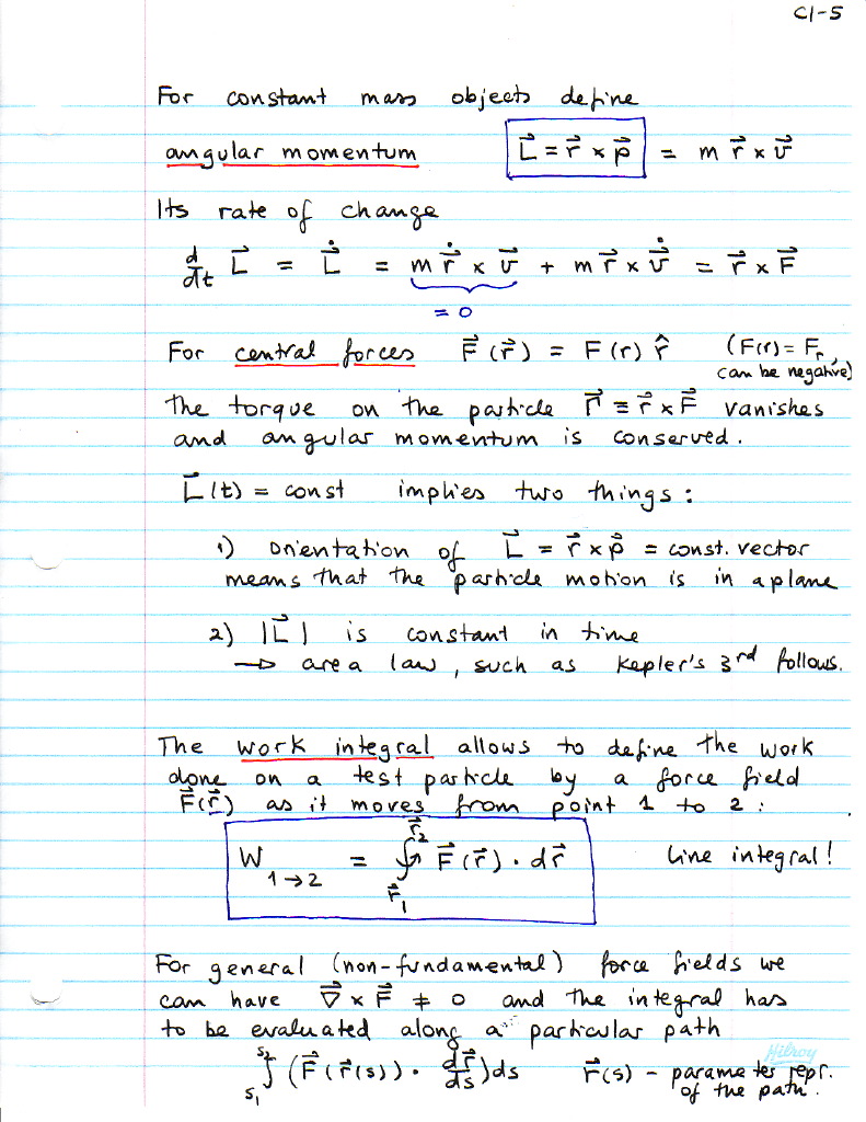
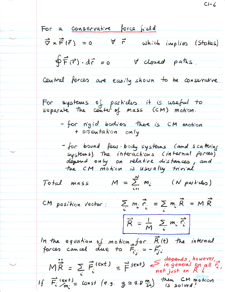
NEWTONIAN MECHANICS
1.1 Introduction 1.1 Intro-2 1.1 Intro-3
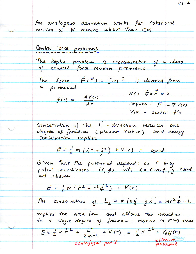
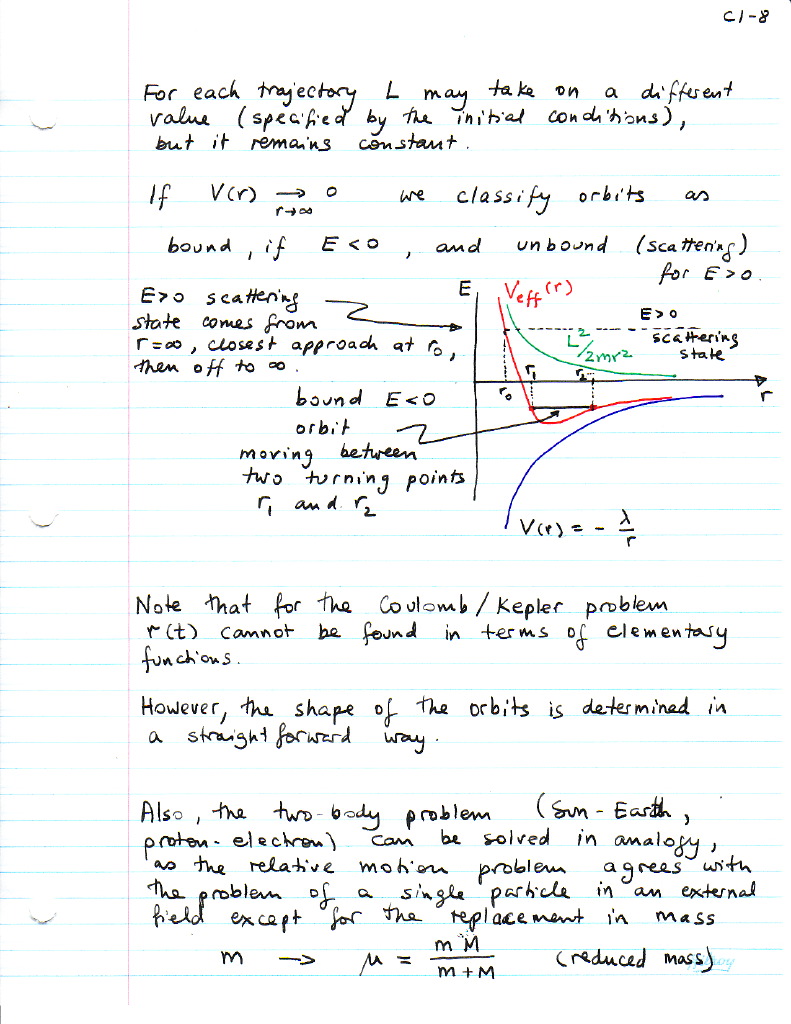
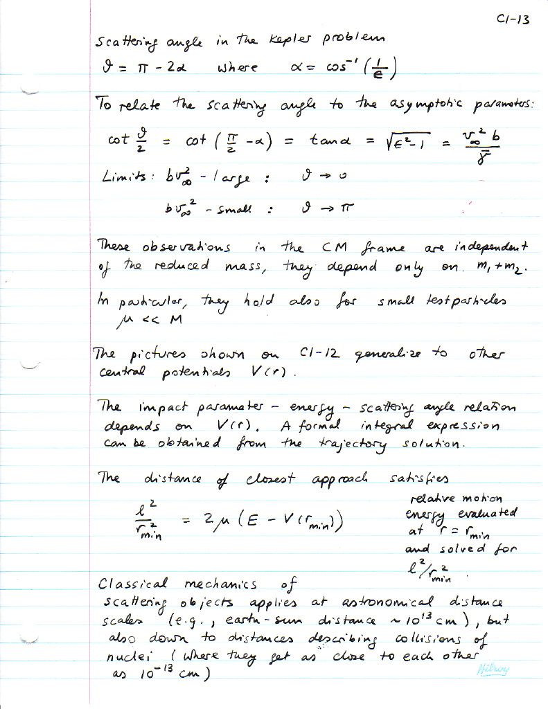
1.3 Scattering orbits Sc-2 Sc-3 Sc-4 Sc-5
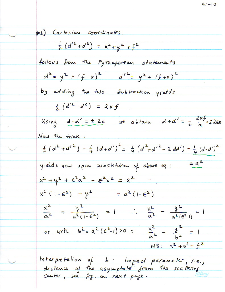
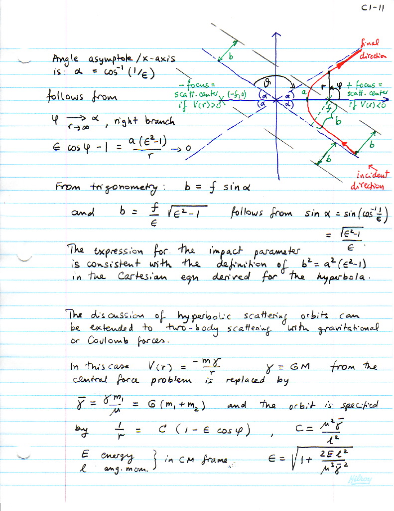
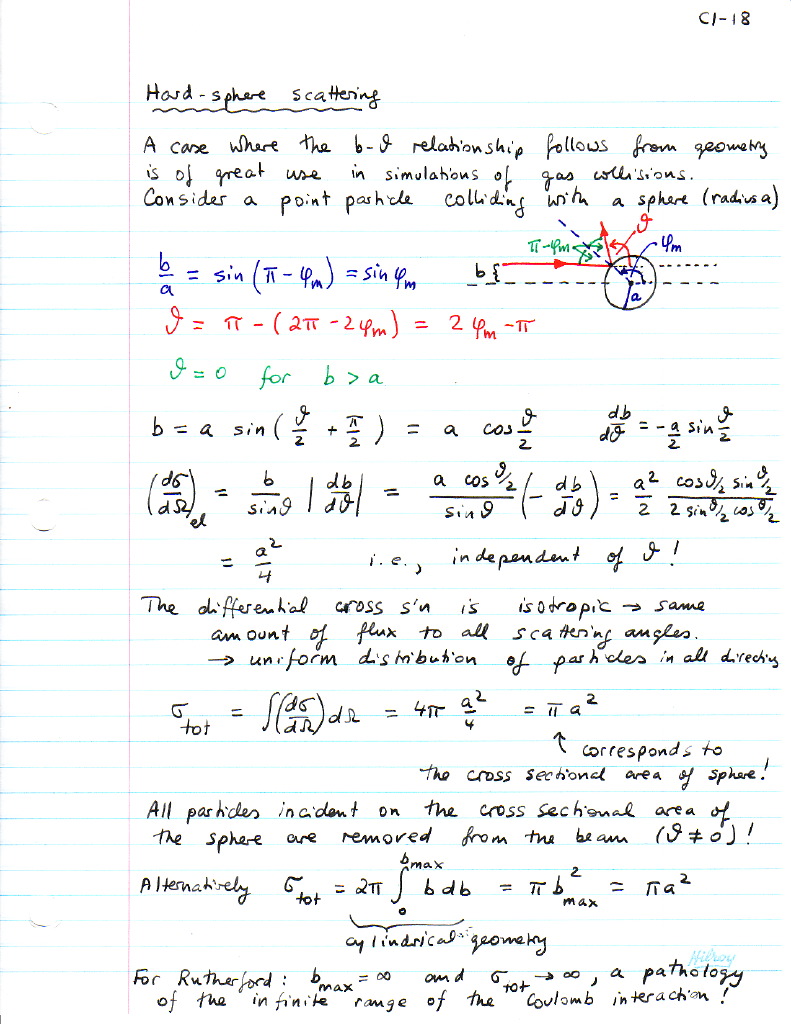
1.3 Rutherford scattering Hard-sphere scattering
LAGRANGIAN MECHANICS
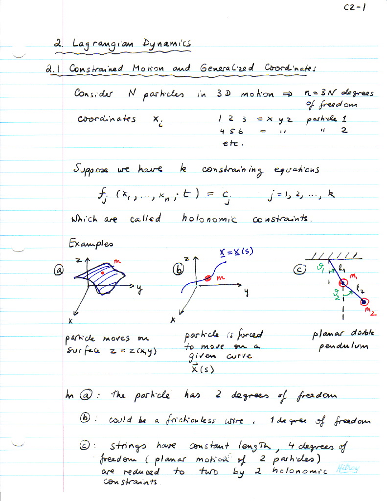
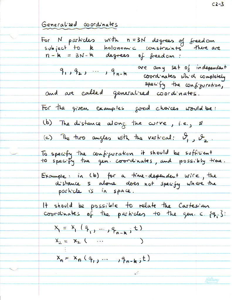
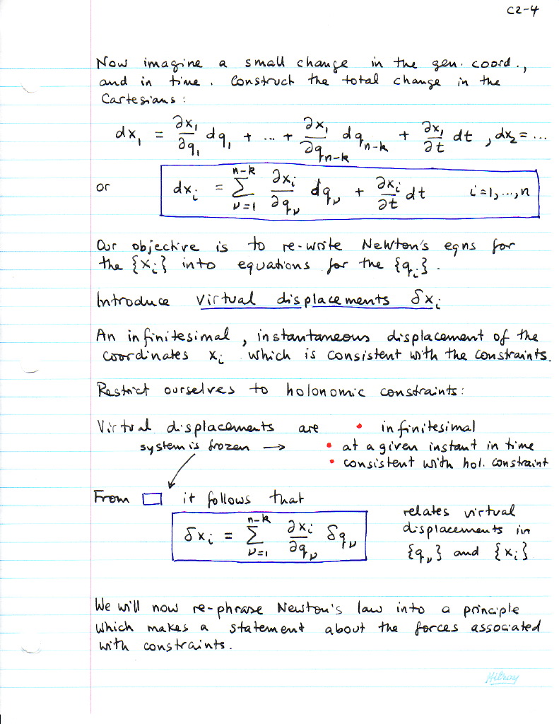
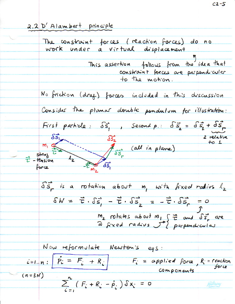
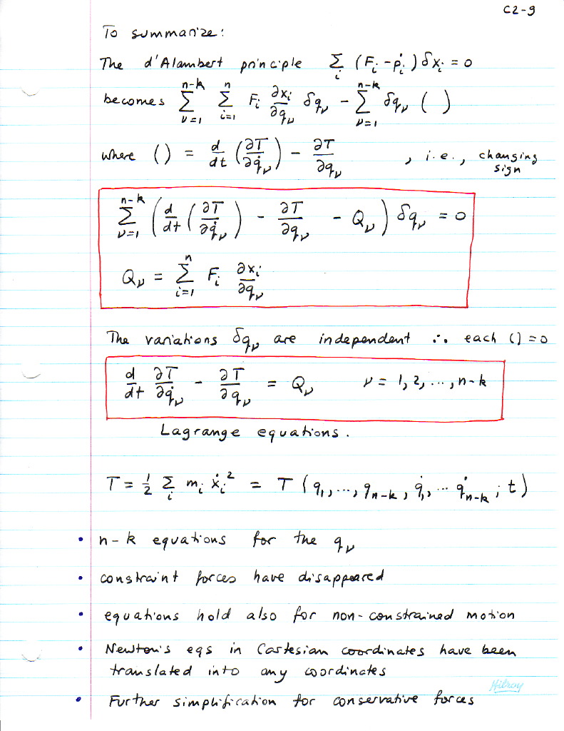
2.1 Generalized coordinates Gc-2 2.2 D'Alambert principle
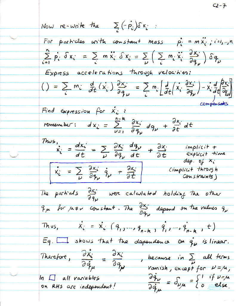
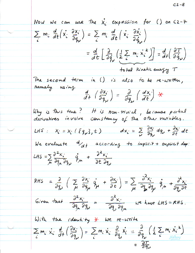
2.3 Lagrange's equations Le-2 Le-3 Le-4 Le-5
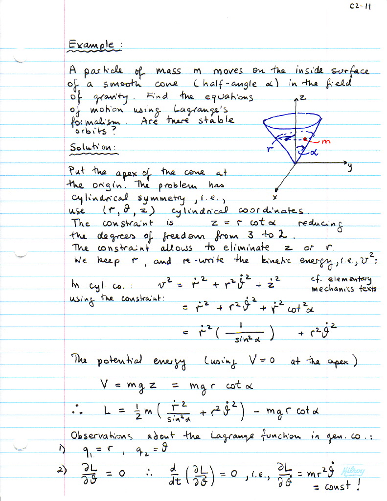
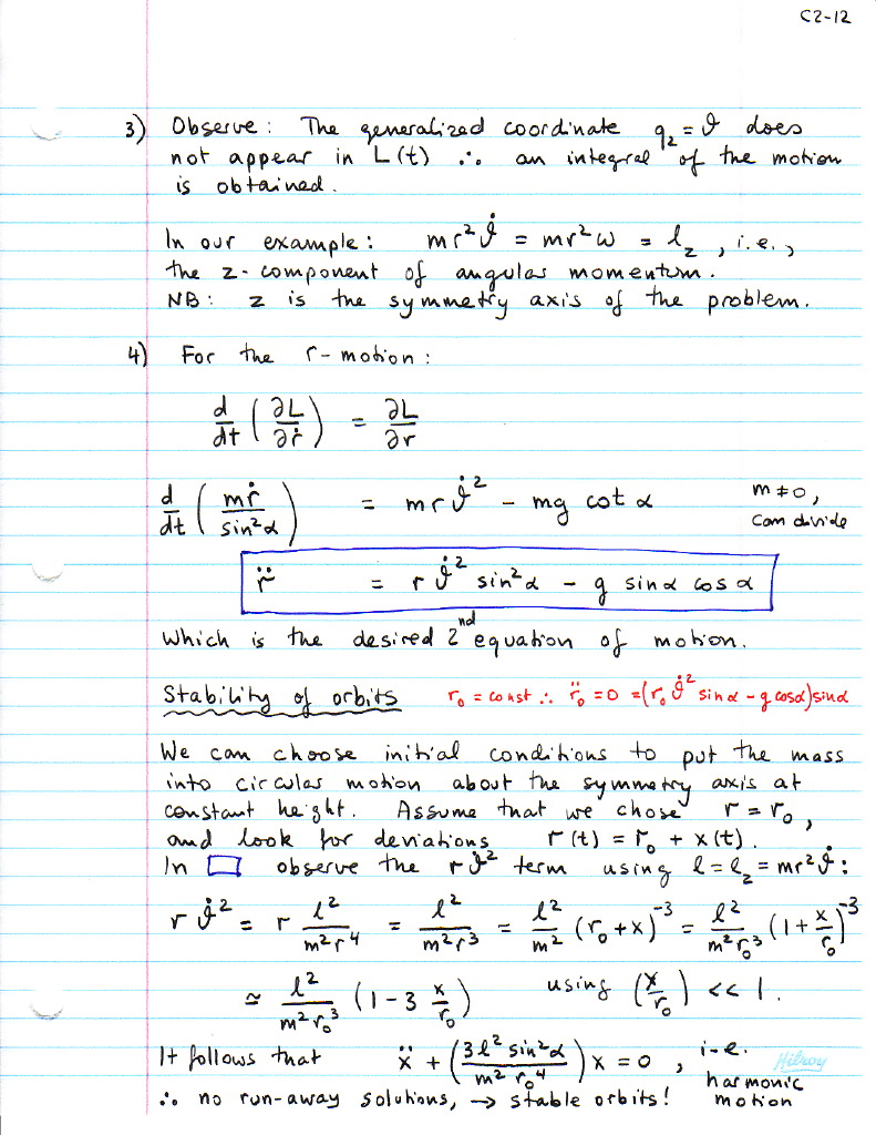
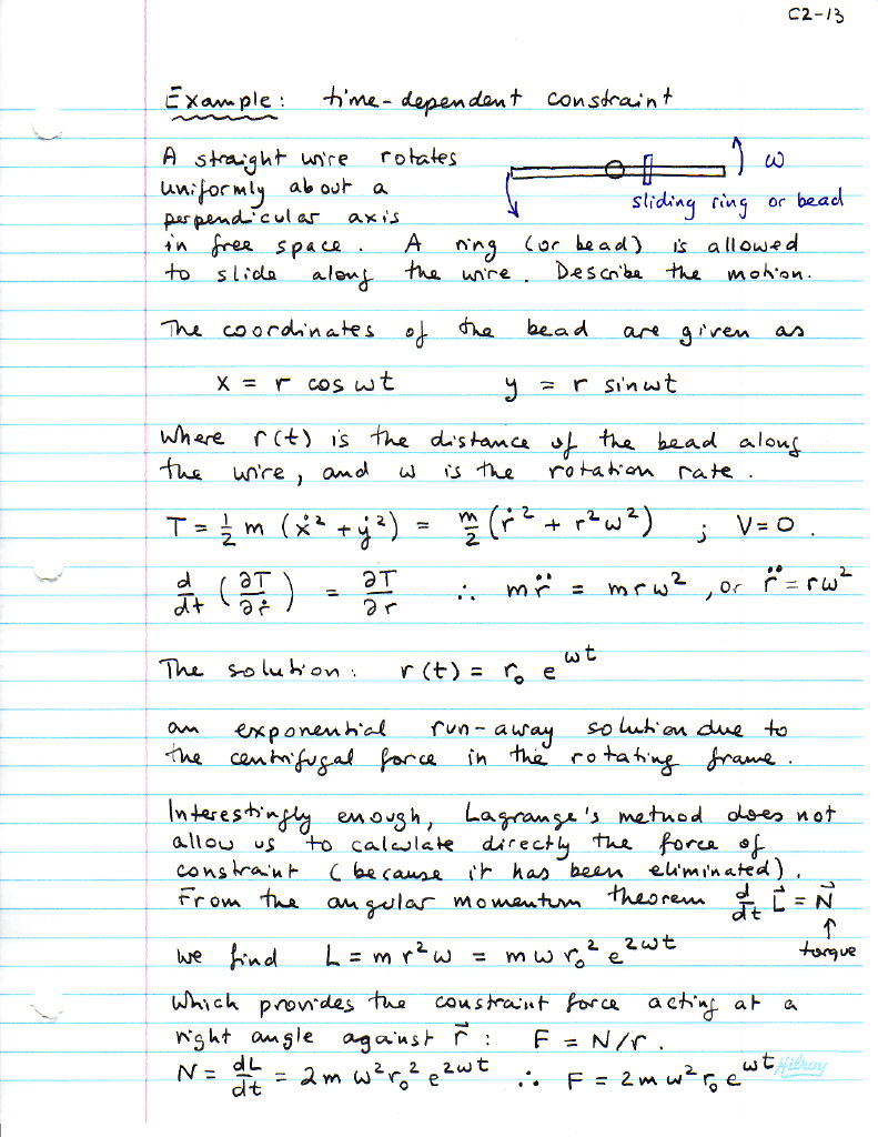
2.3 Example 1 Ex.1-2 Example 2
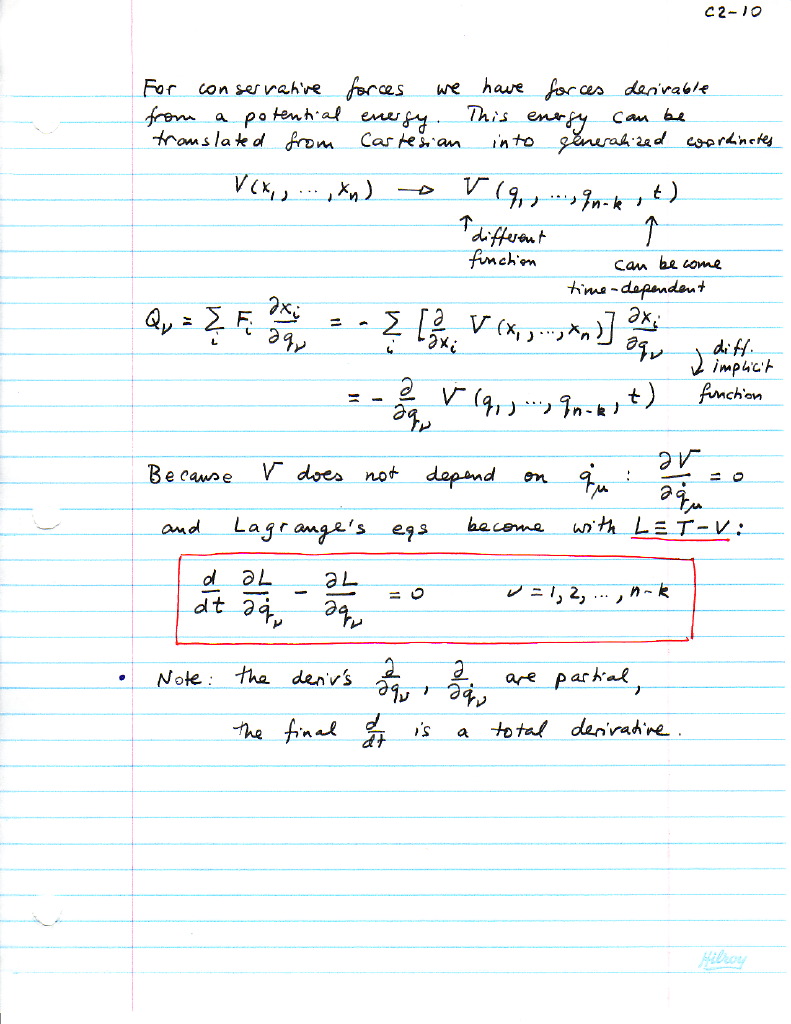
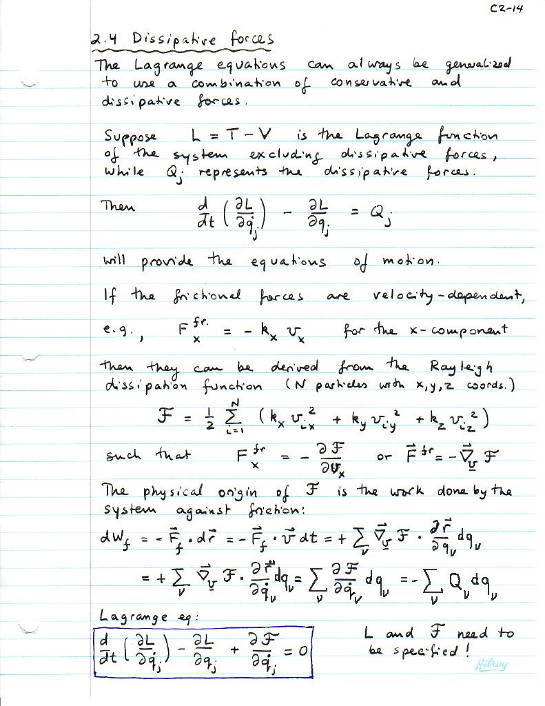
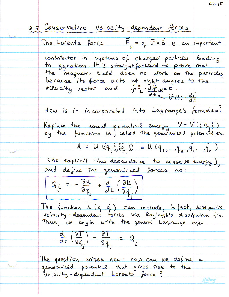
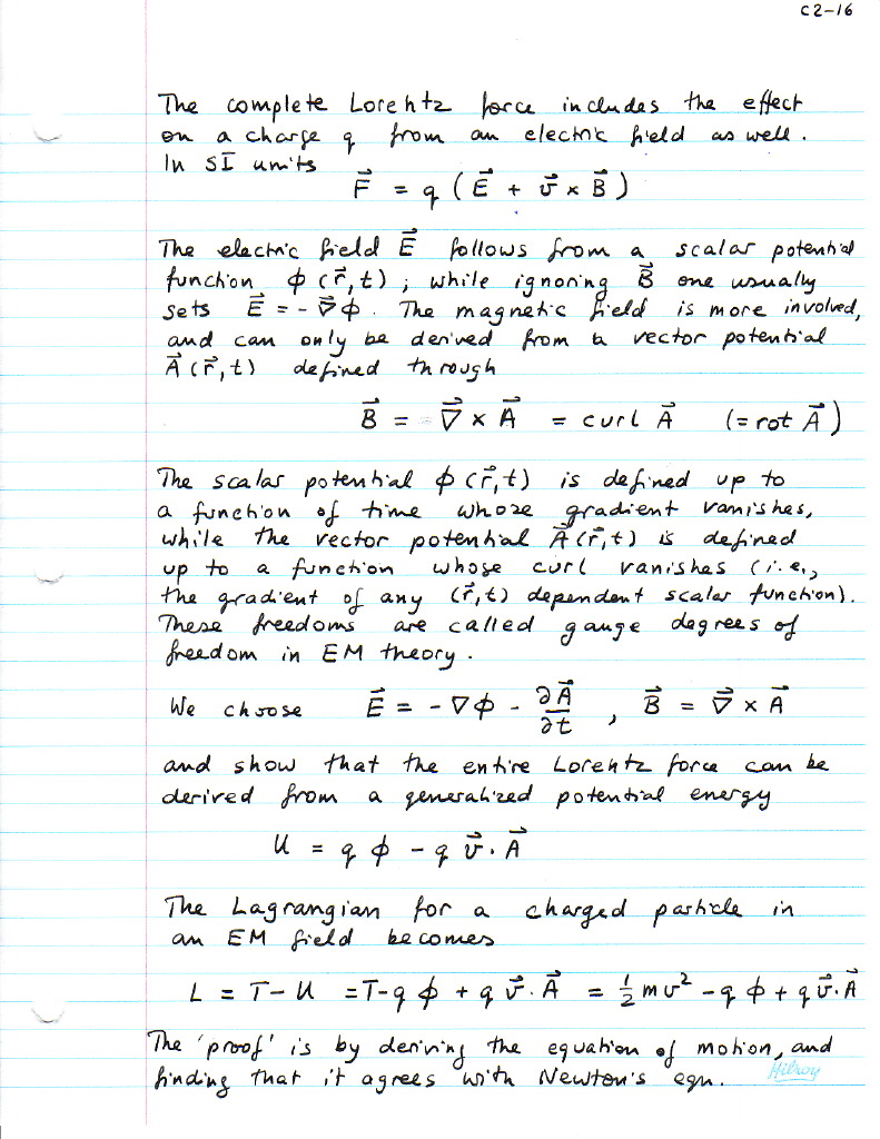
2.4 Dissipative forces 2.5 Conservative velocity-dep forces 2.5 Lorentz force Lf-2
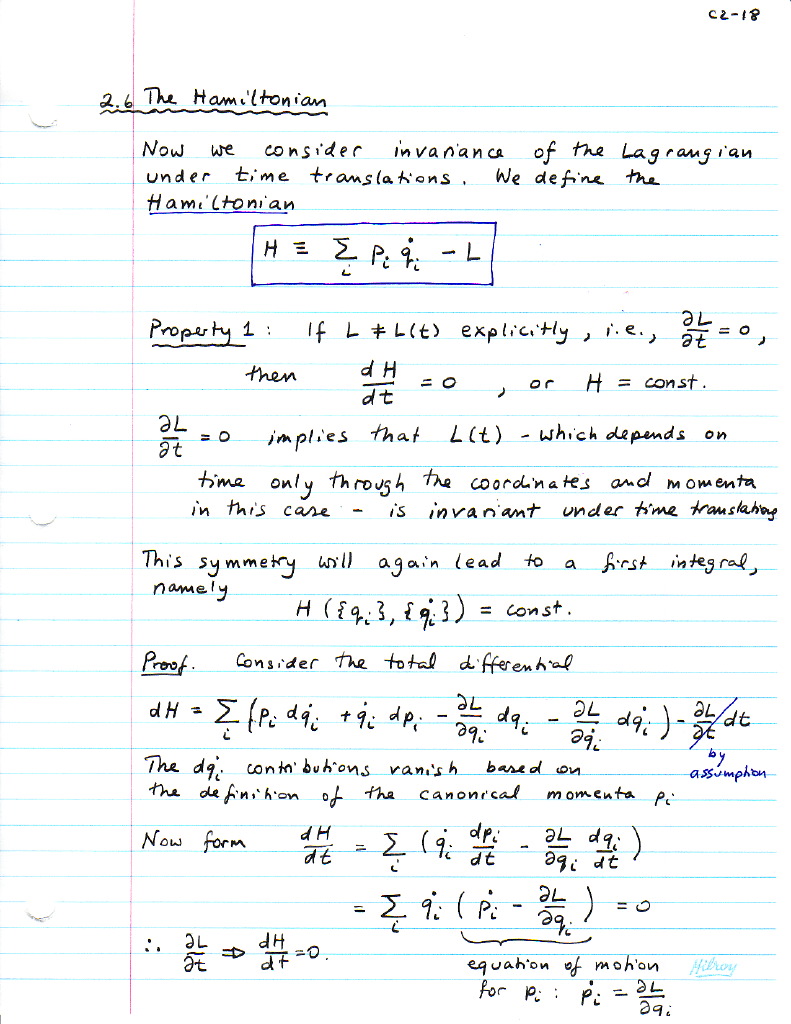
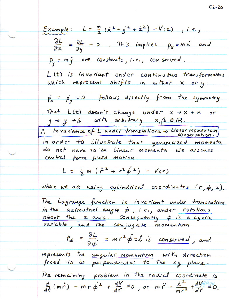
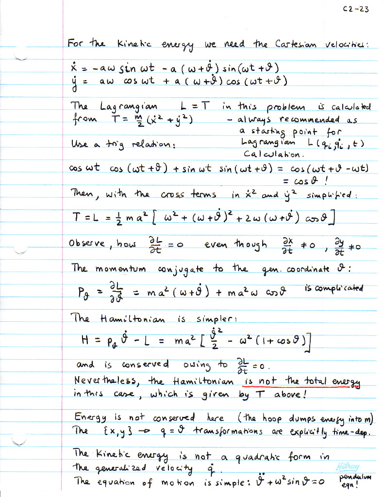
2.6 The Hamiltonian 2.6 Generalized momentum 2.6 Conservation laws
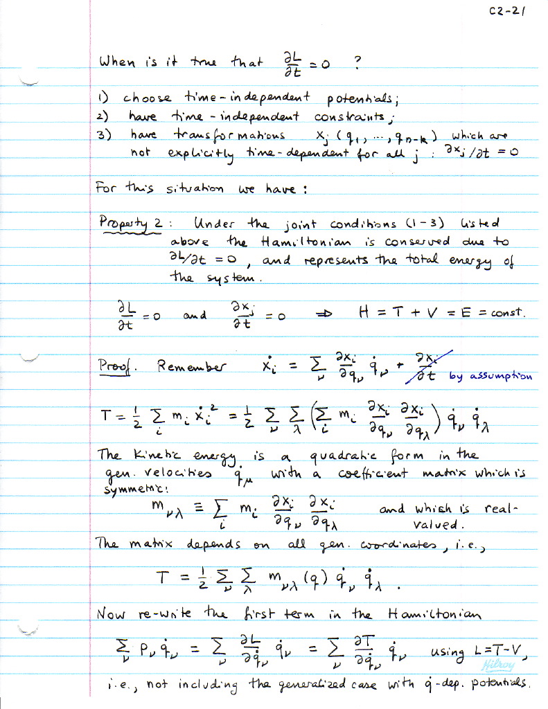
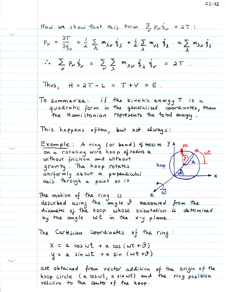
2.6 The Energy 2.6 Example Ex-1
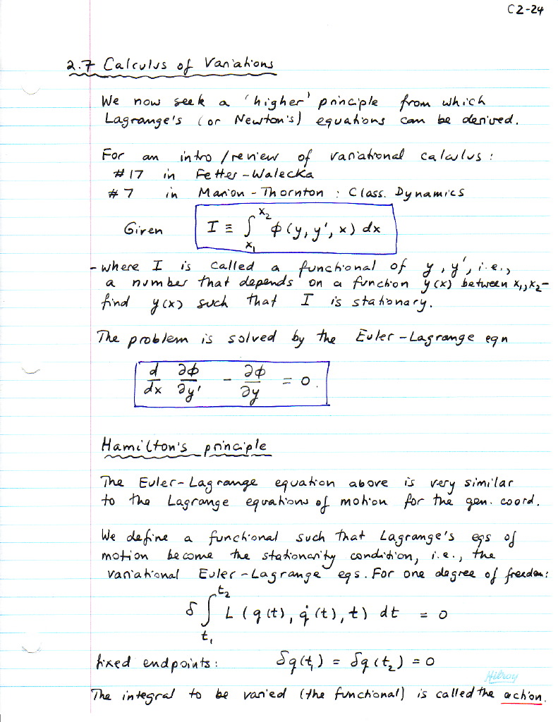
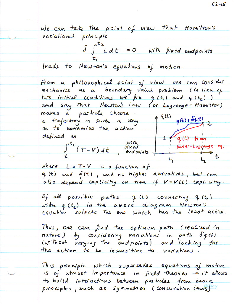
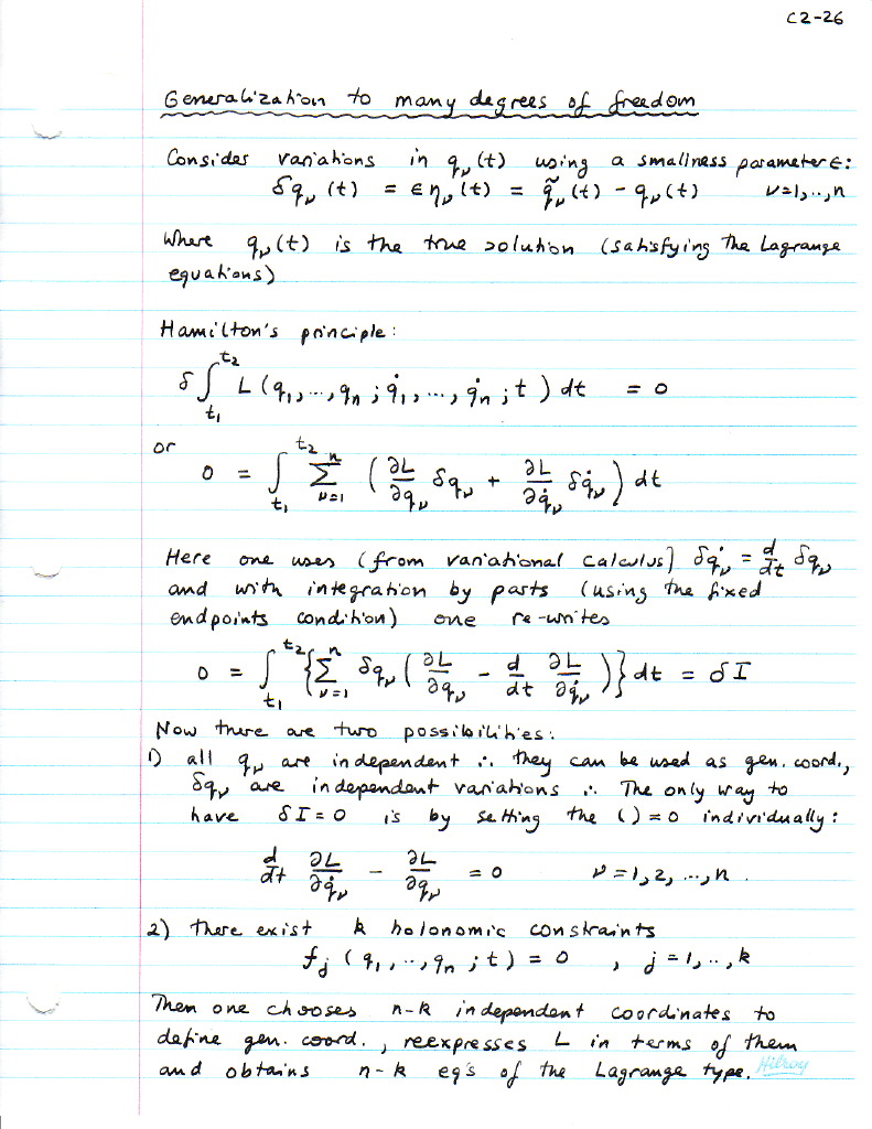
2.7 Hamilton's variational principle HVP-2 2.7 Many degrees of freedom
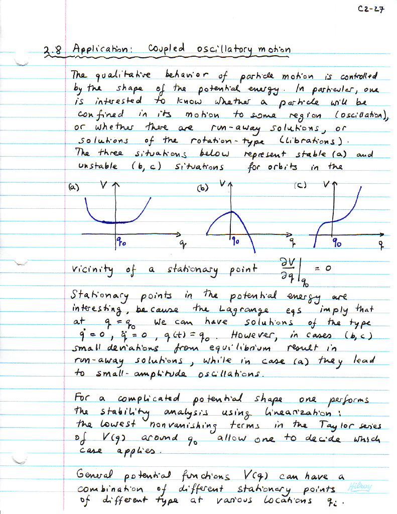
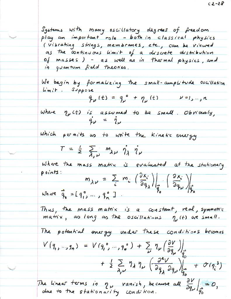
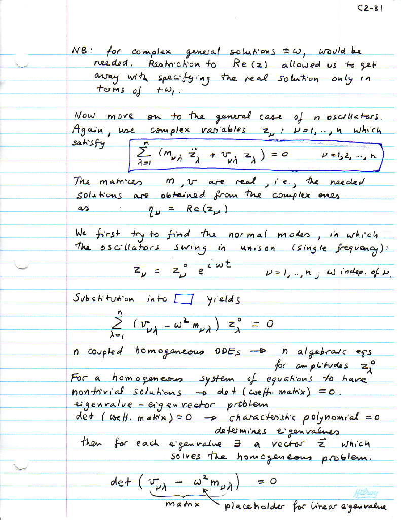
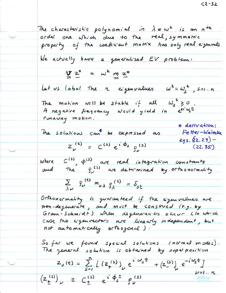
2.8 Coupled oscillatory motion COM-2 COM-3
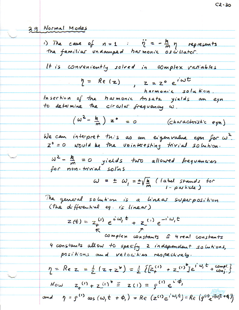
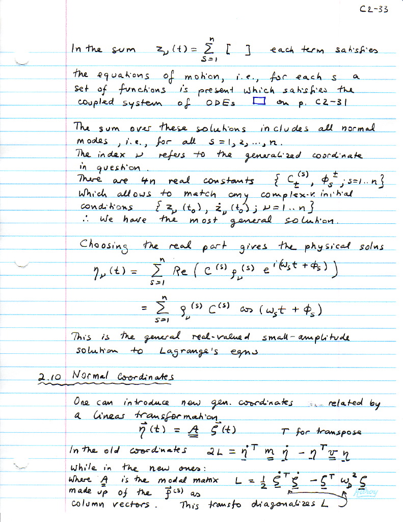
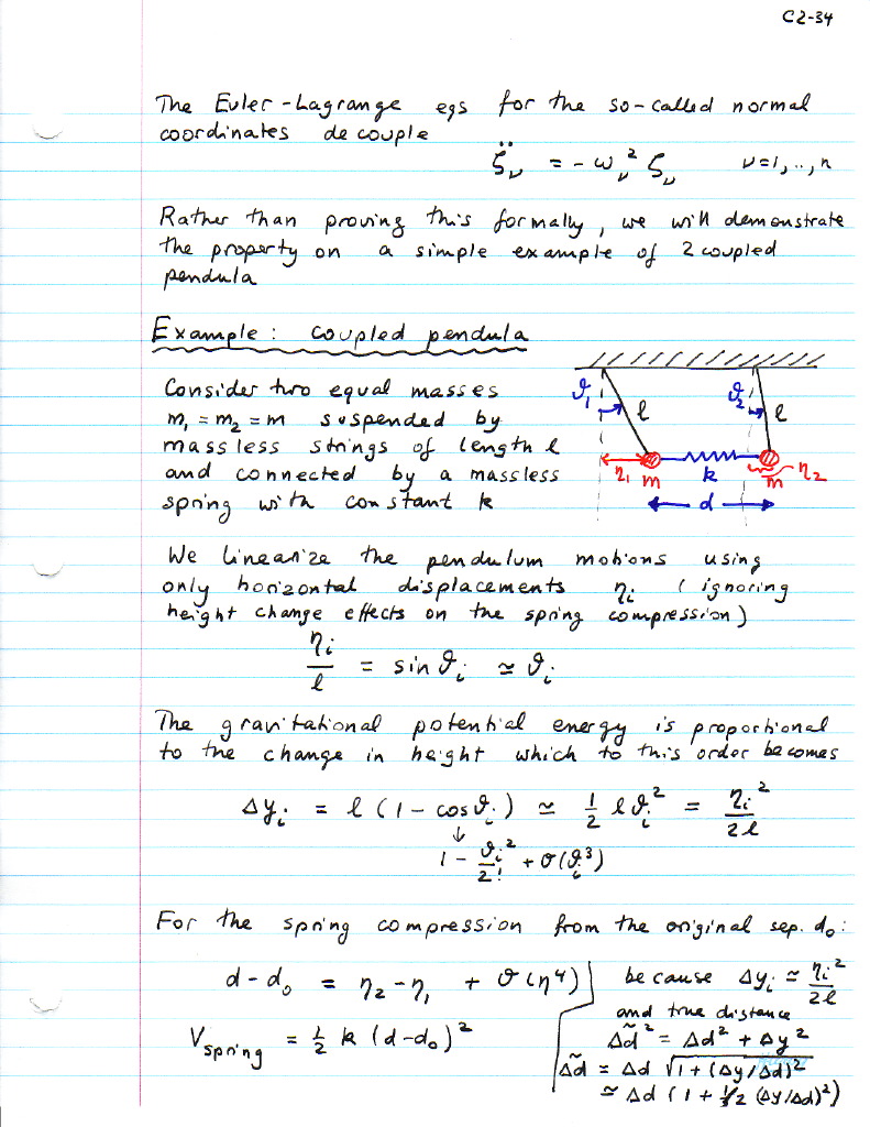
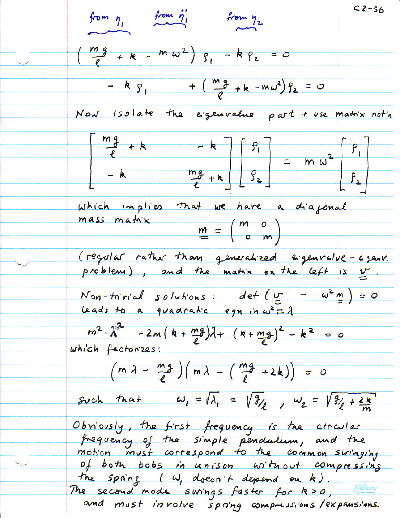
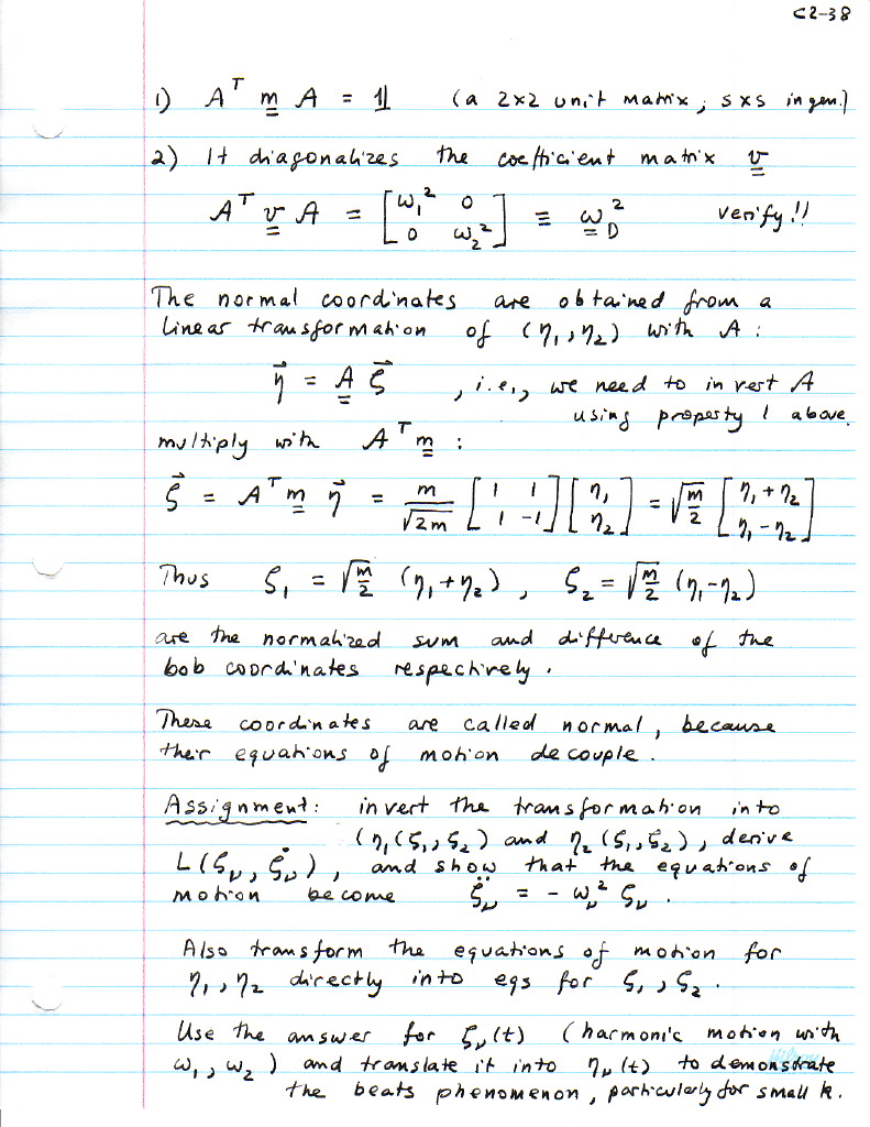
2.10 Normal coordinates: coupled pendula NC-2 NC-3 NC-4 NC-5 NC-6
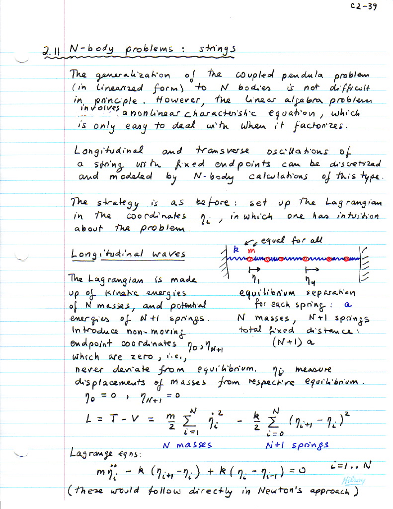
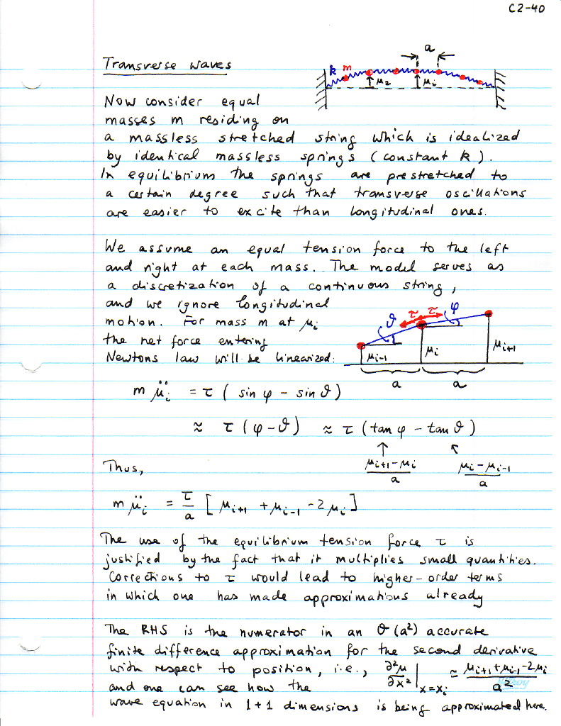
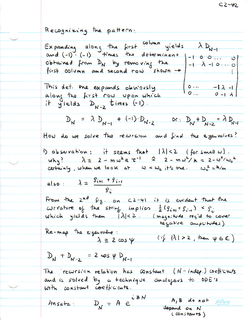
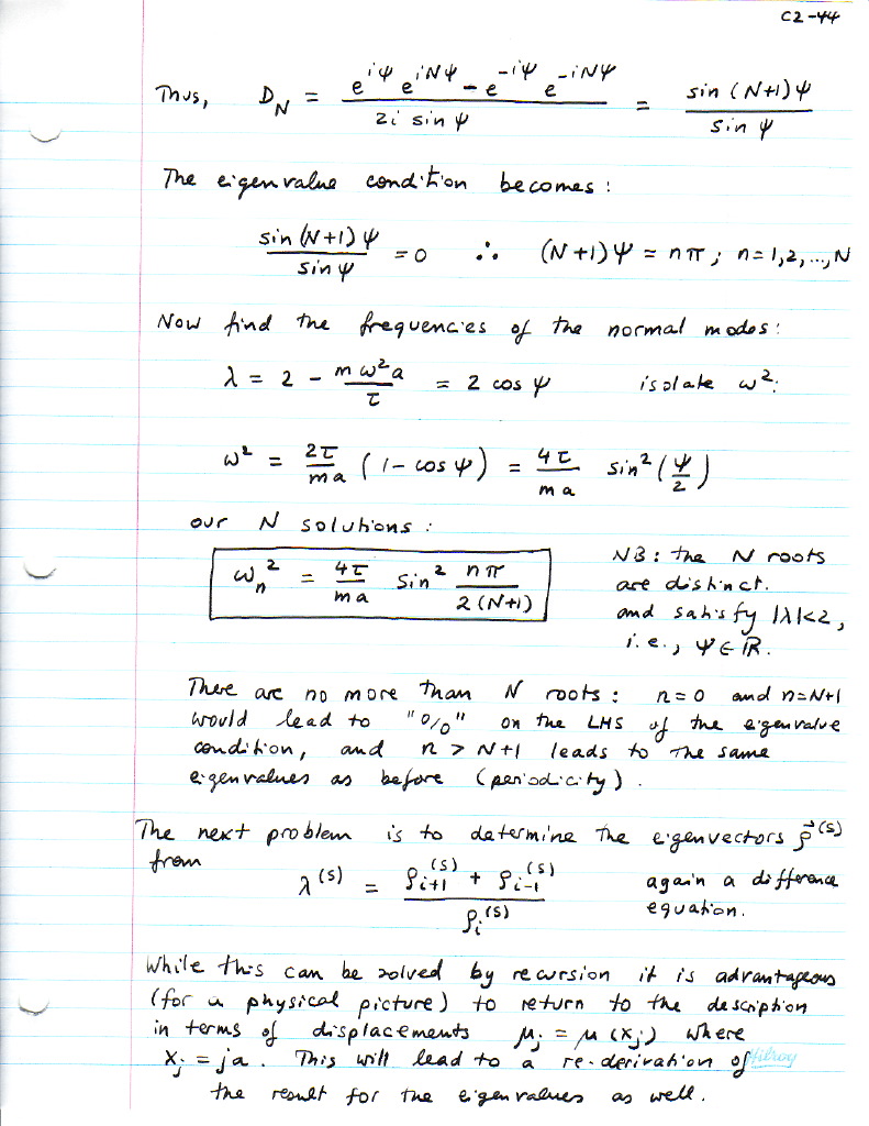
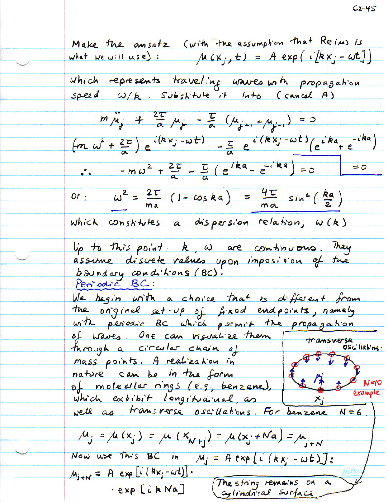
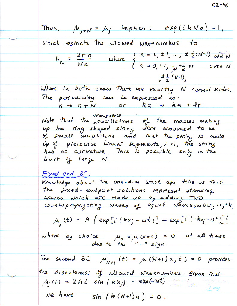
2.11 N-body problems 2.11 Transverse waves TW-2 TW-3 TW-4 TW-5 TW-6 TW-7 TW-8 TW-9
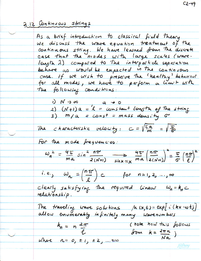
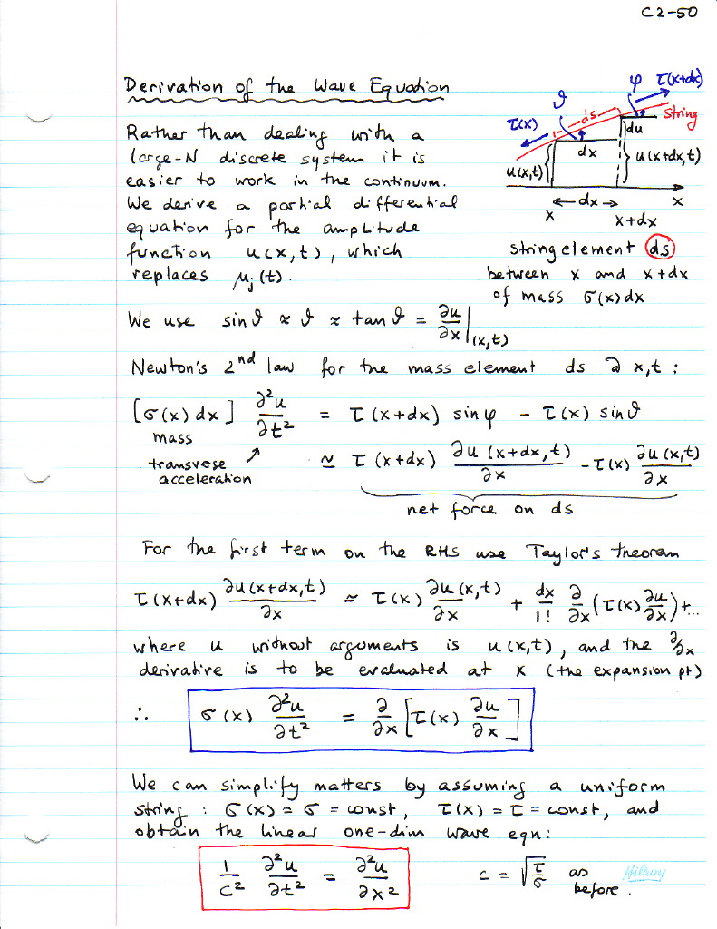
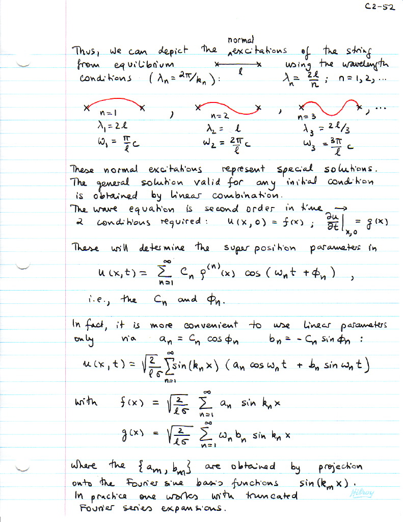
2.12 Continuous strings 2.12 Wave equation WE-2 WE-3
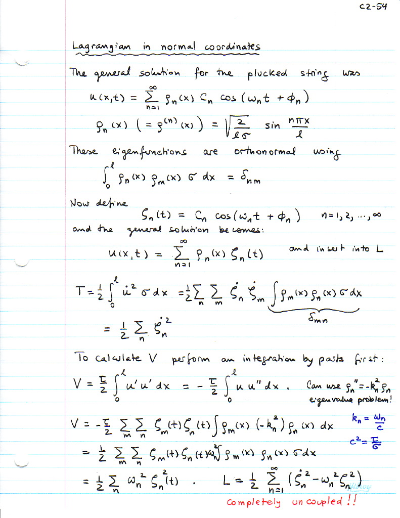
2.13 Lagrangian for a continuous string LCS-2
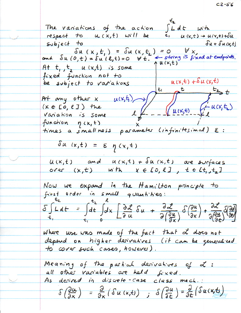
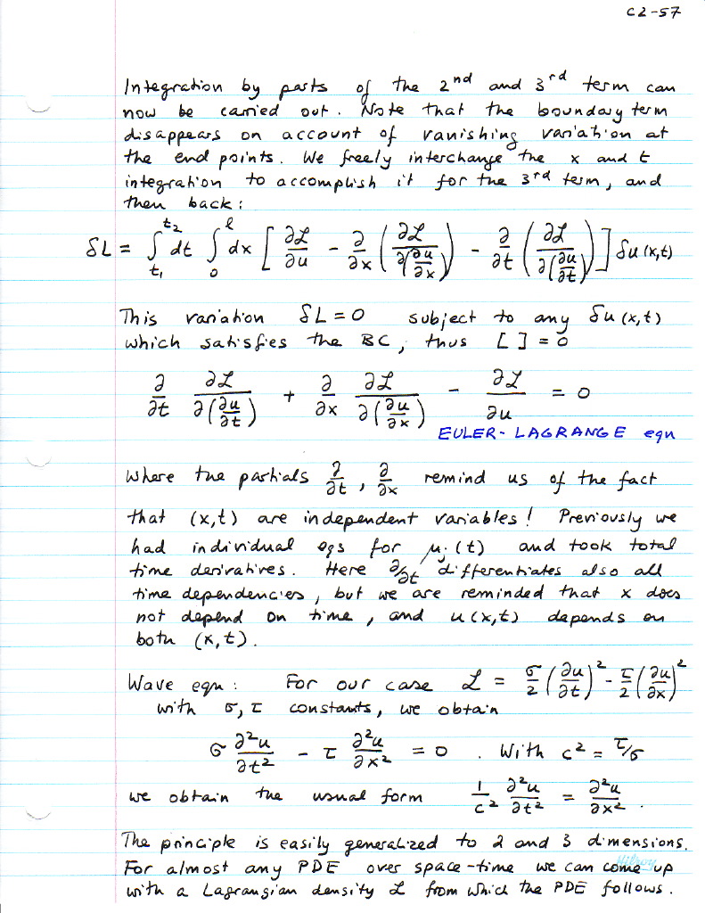
2.14 Hamilton's principle HP-2 HP-3
HAMILTONIAN MECHANICS
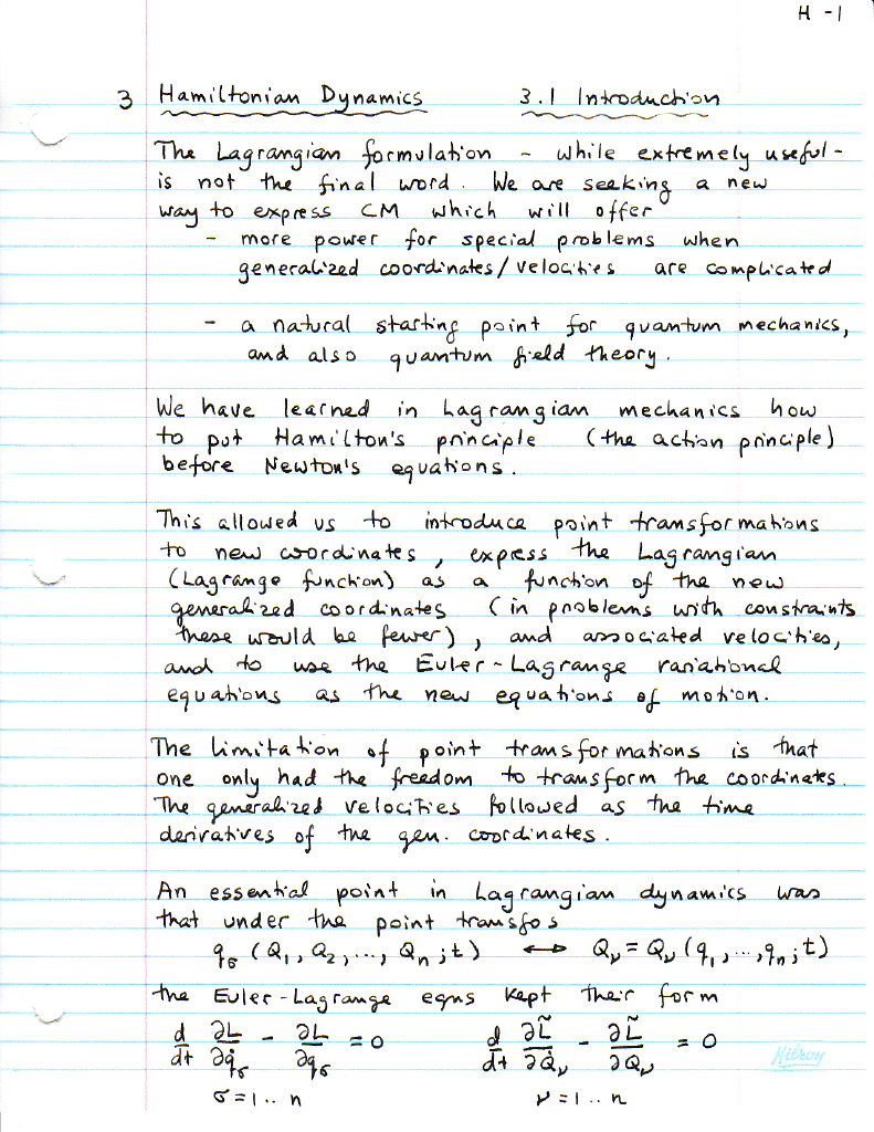
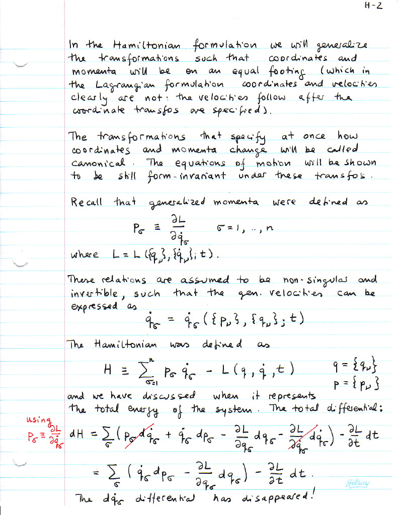
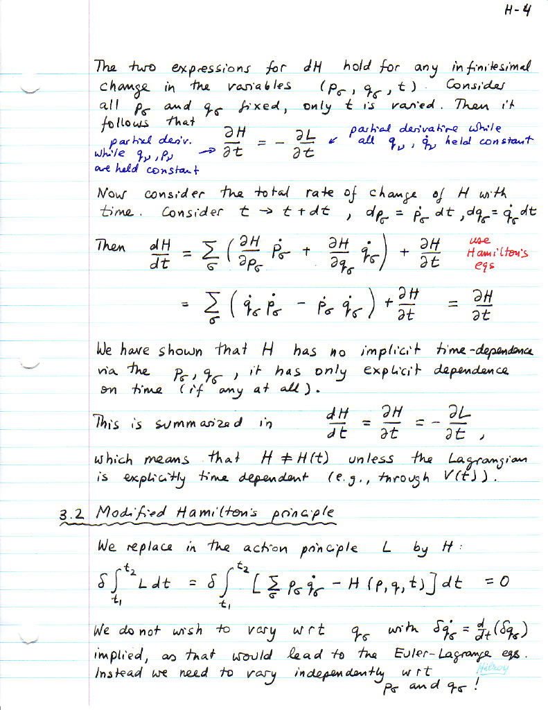
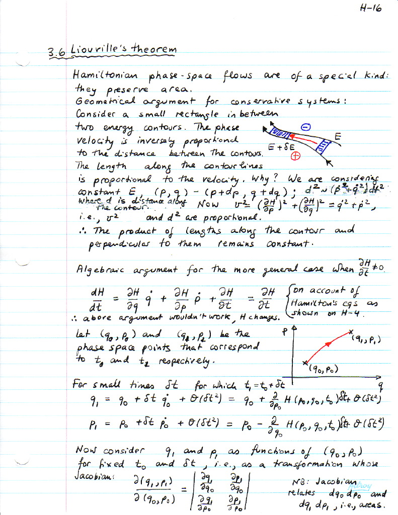
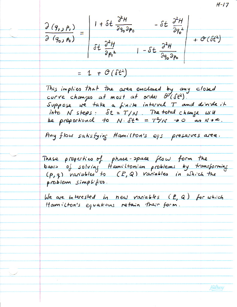
3.1 Hamilton's equations H-2 H-3
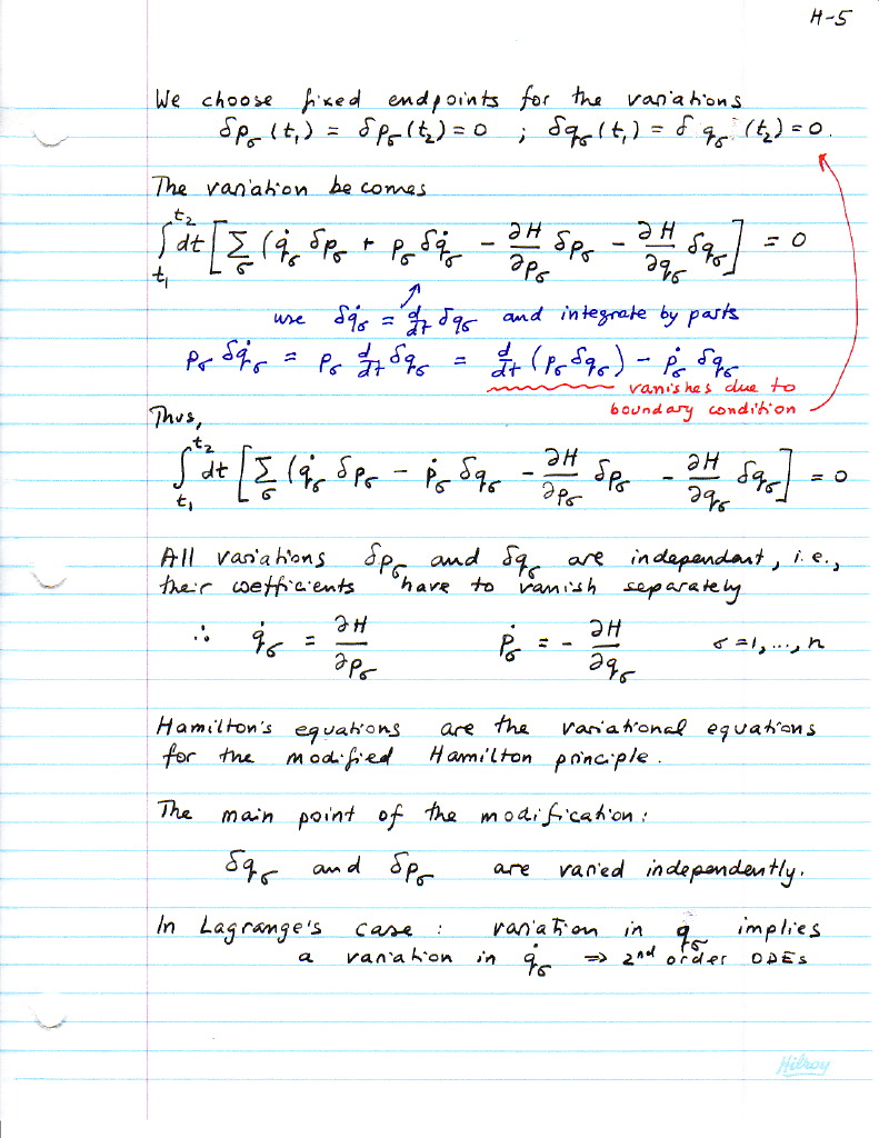
3.2 Modified Hamilton's principle H-2
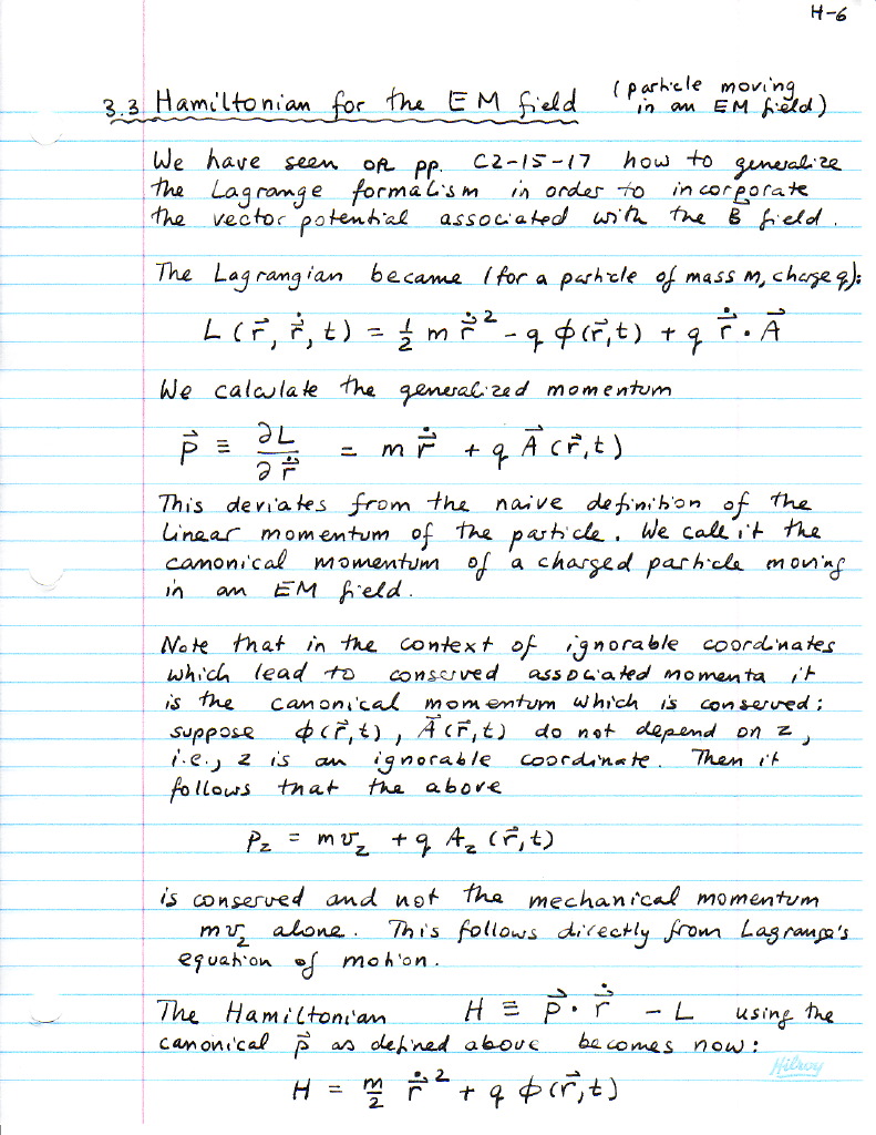
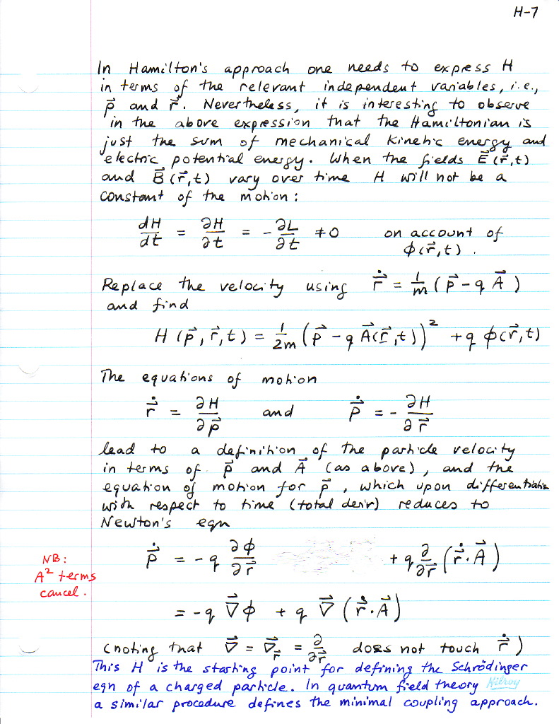
3.3 Hamiltonian for the EM field HEM-2
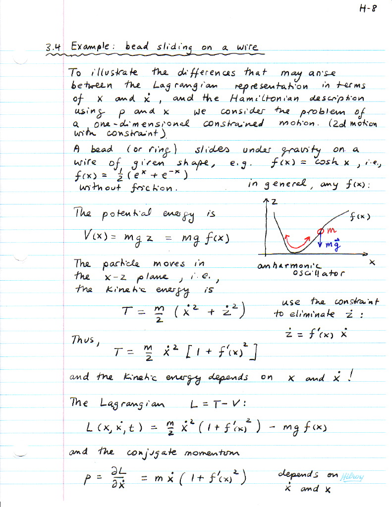
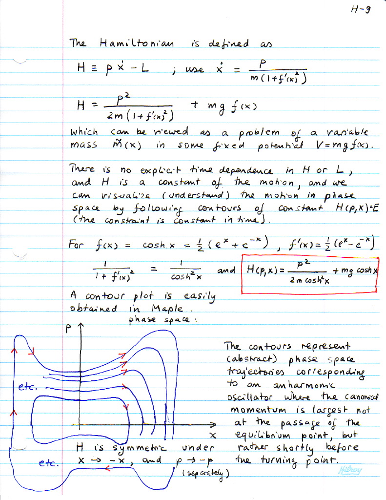
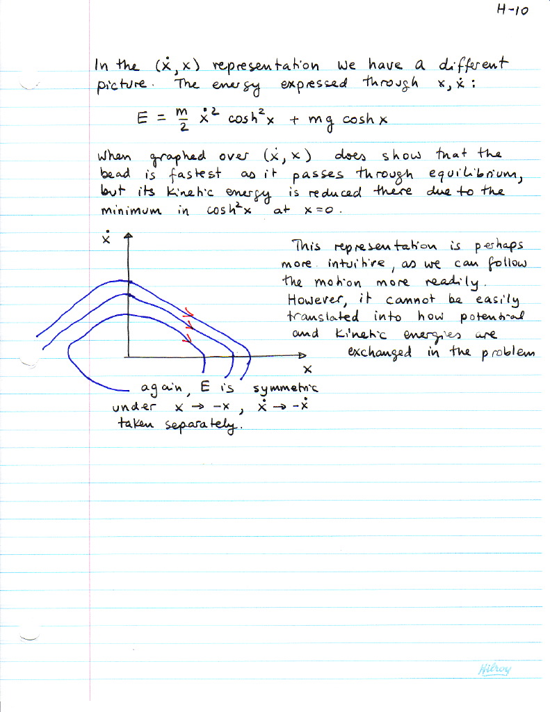
3.4 Example: bead on a wire B-2 B-3
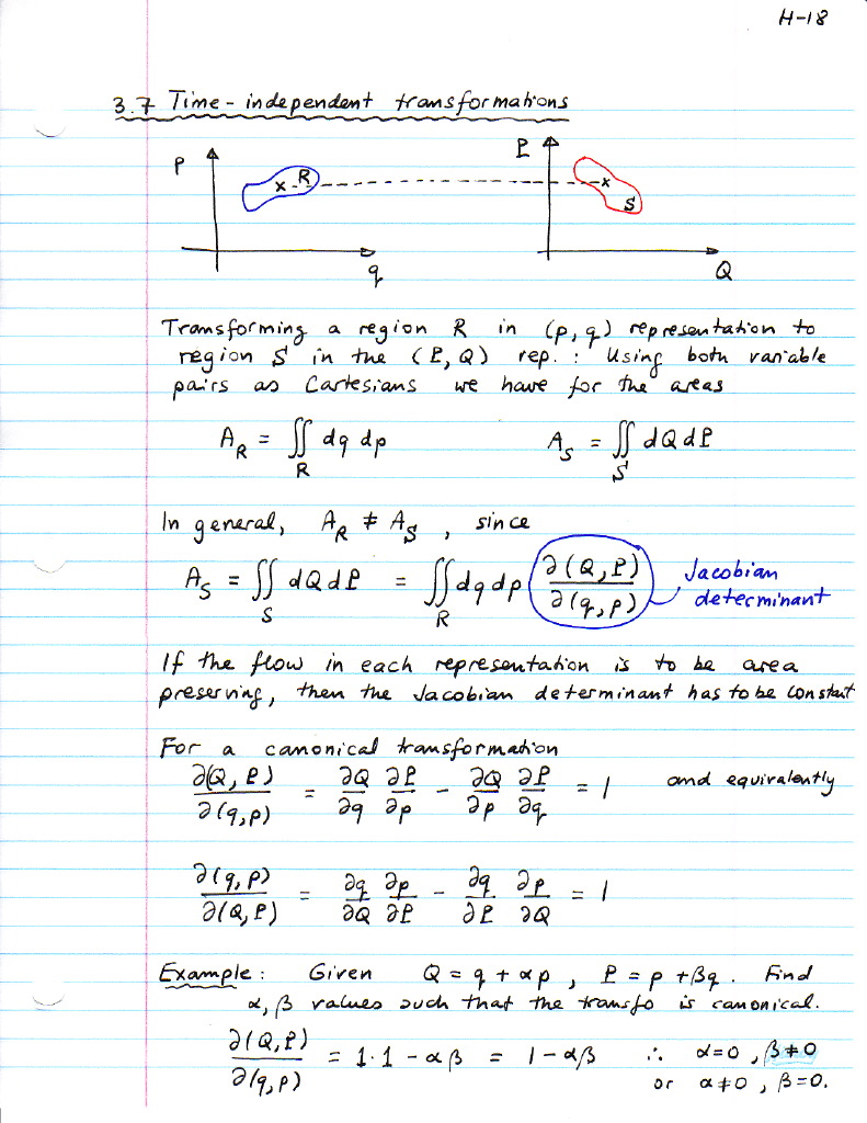
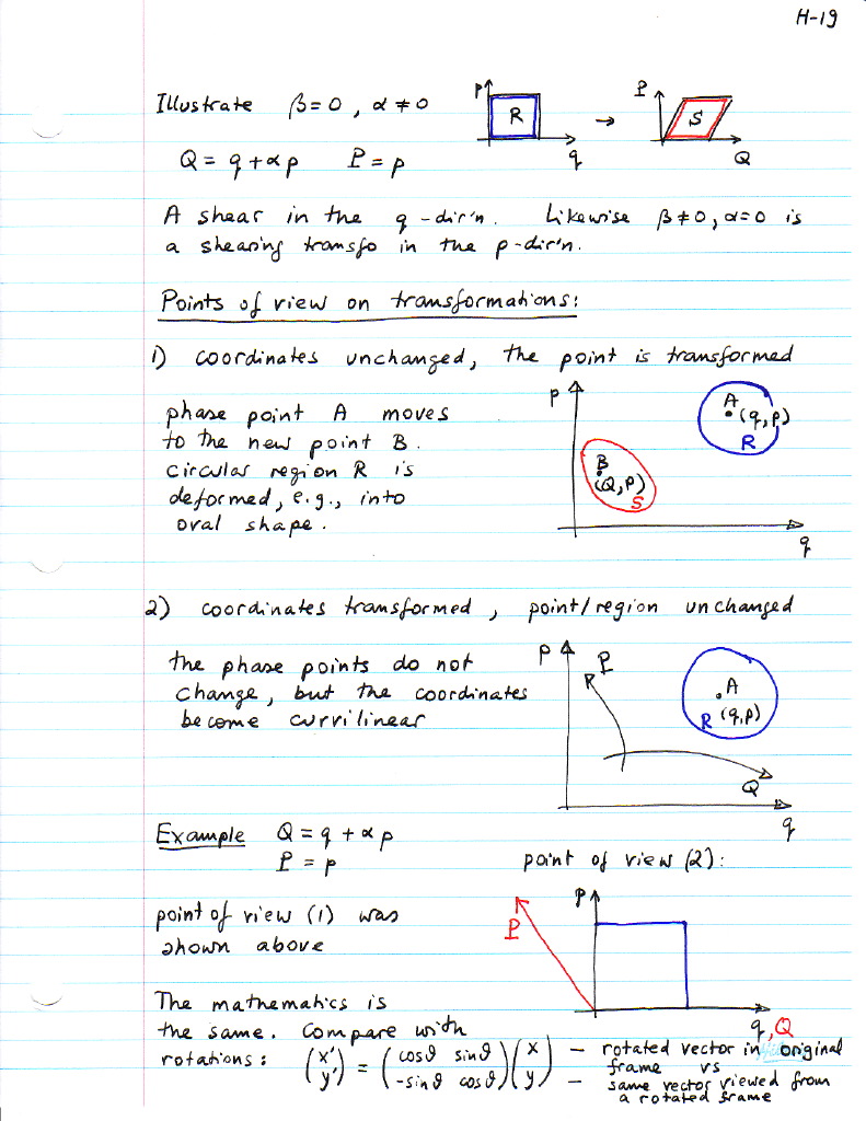
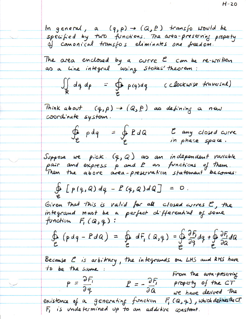
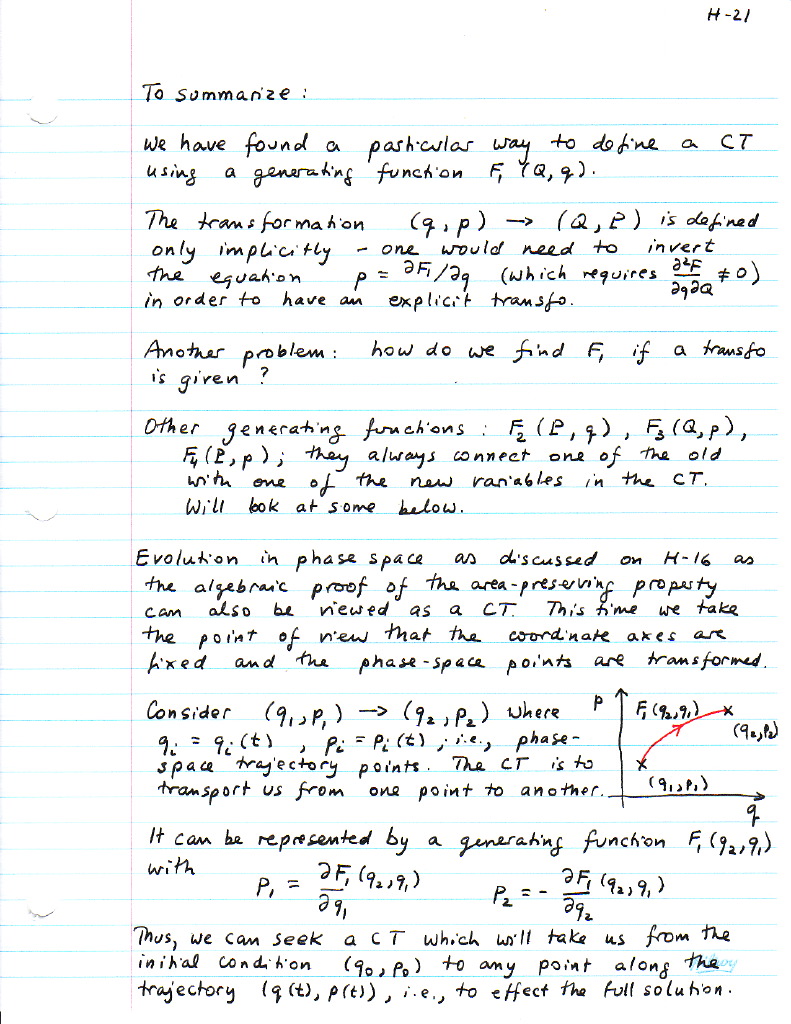
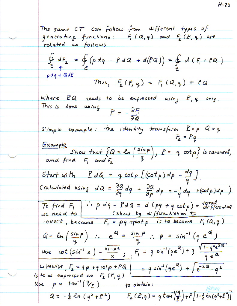
3.7 Canonical transformation CT-2 CT-3 CT-4
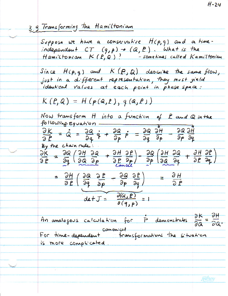
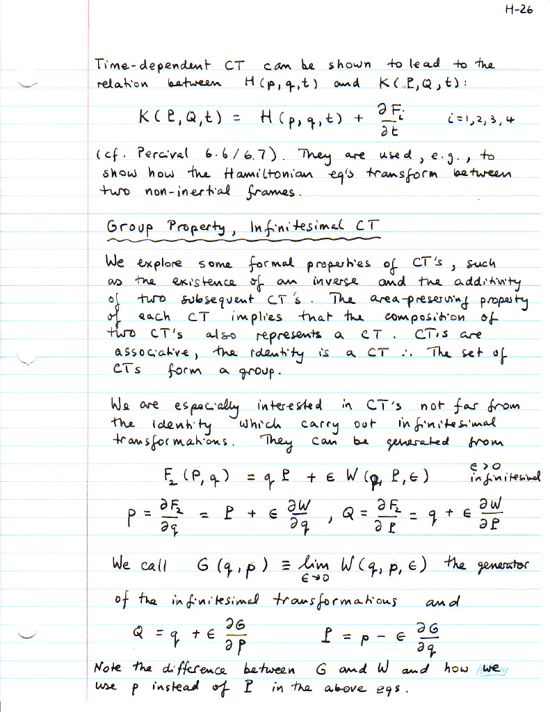
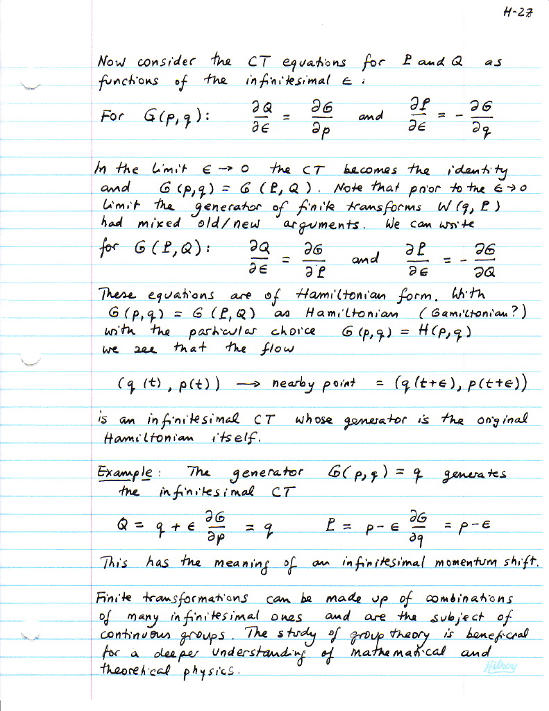
3.9 Transforming the Hamiltonian Example: harmonic osc Infinitesimal CT ICT-2
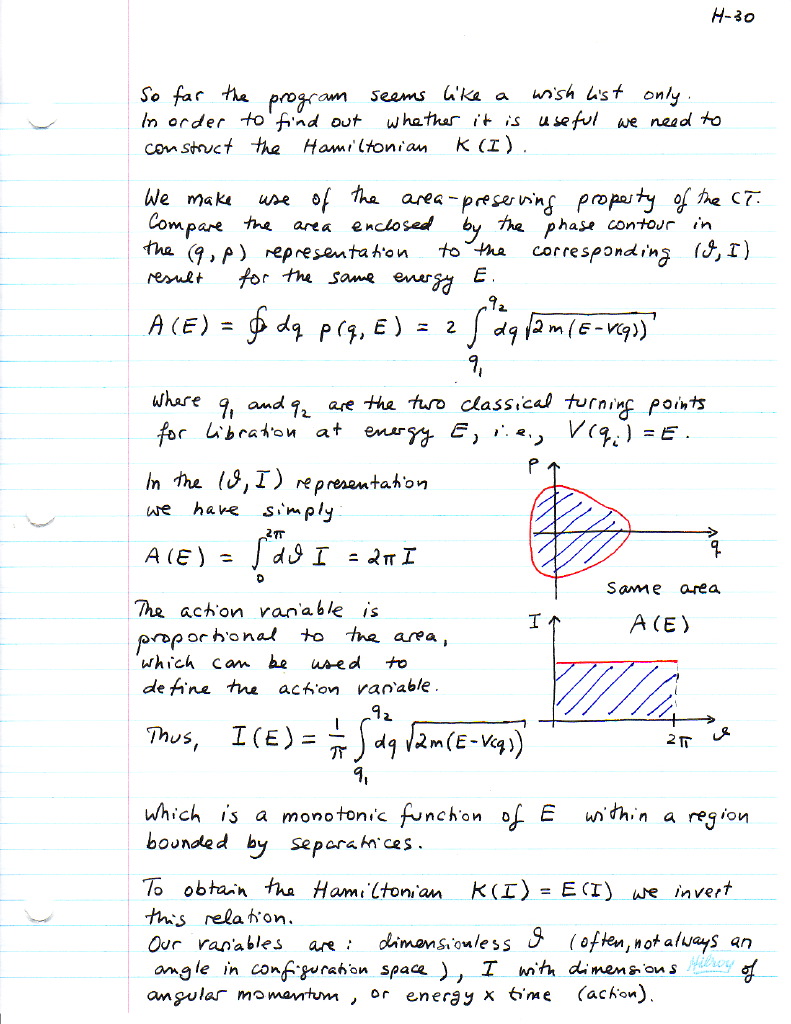
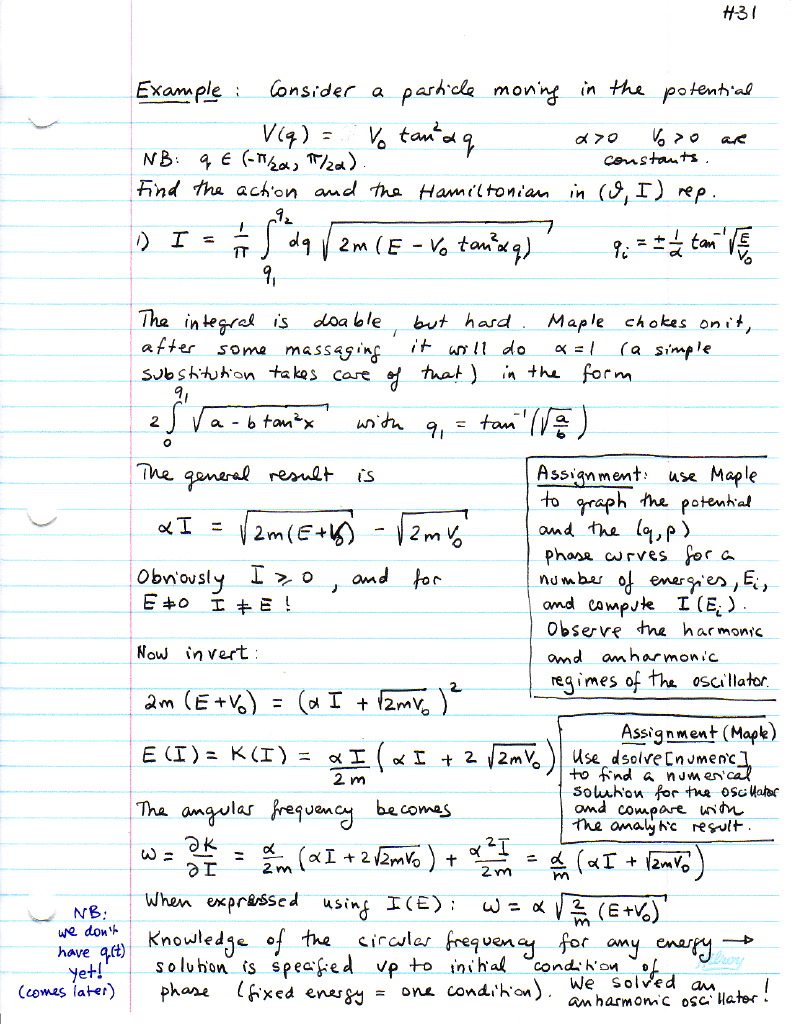
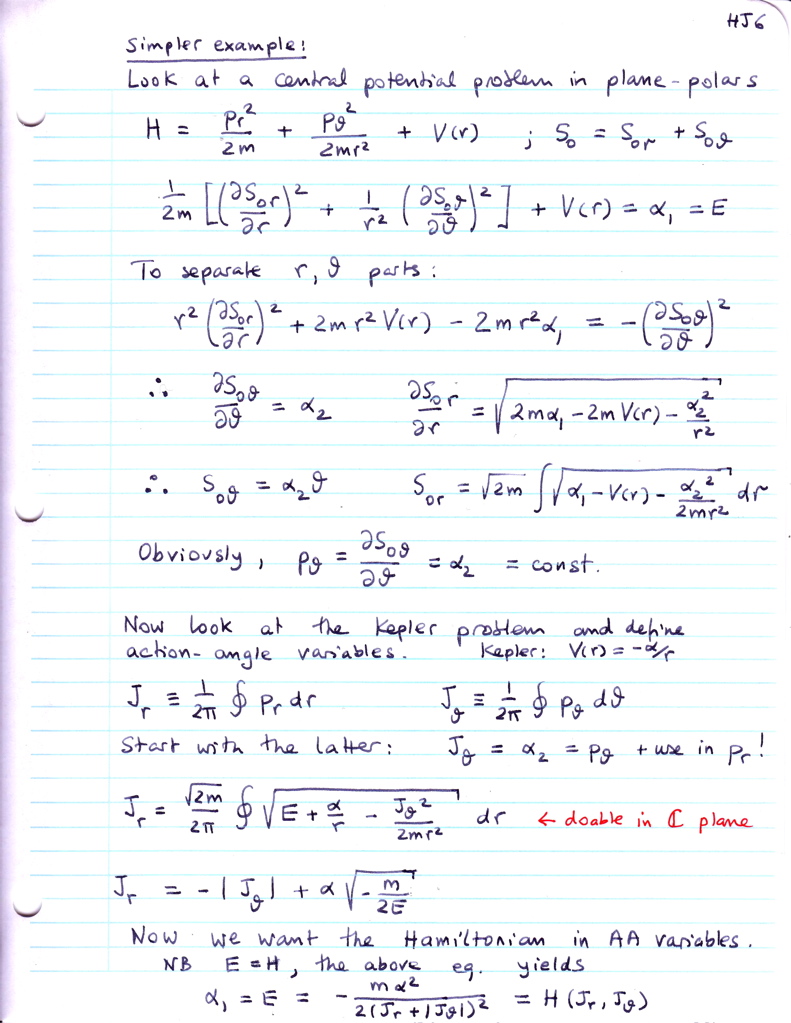
3.10 Action-angle variables AA-2 AA-3
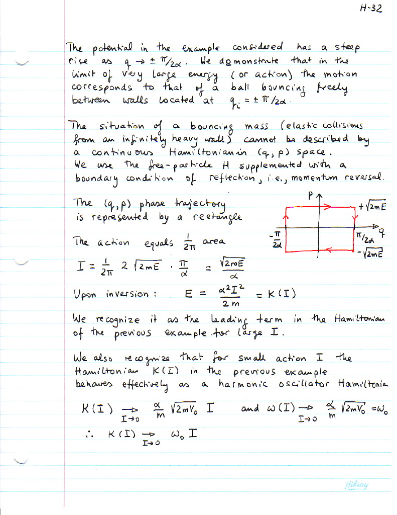
3.11 Solving for the trajectory Example
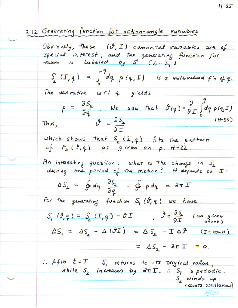
3.12 Generating function for Action-Angle variables
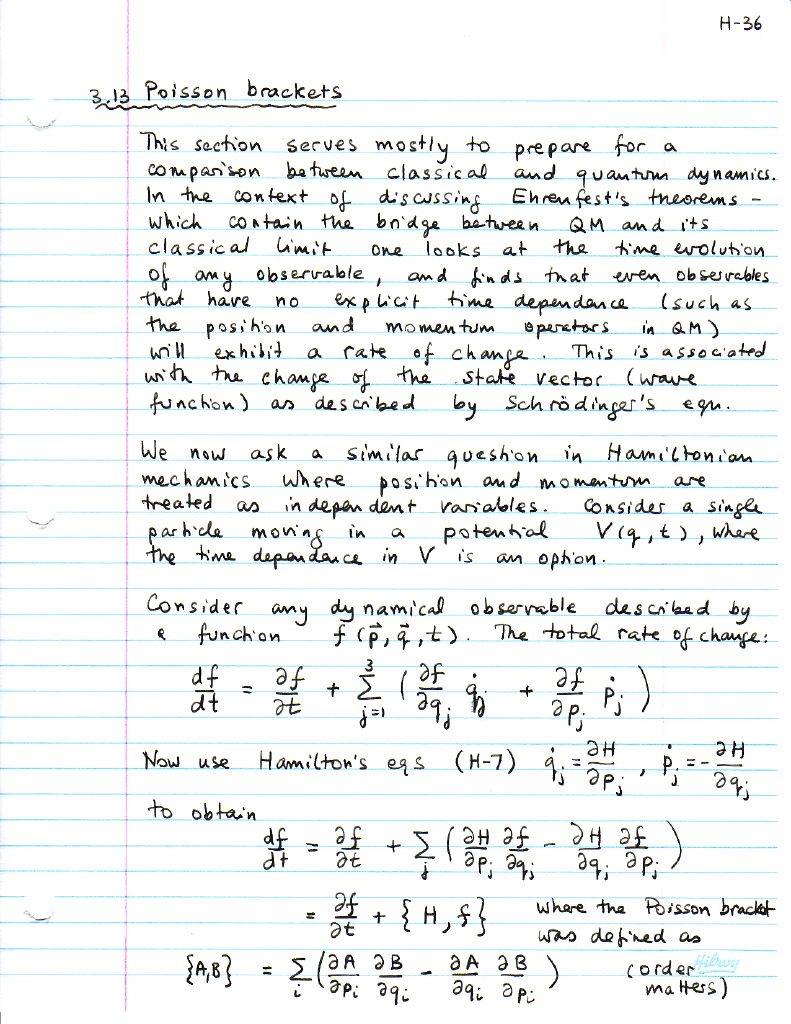
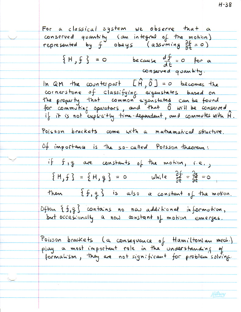
3.13 Poisson brackets Quantum vs Classical QC-2
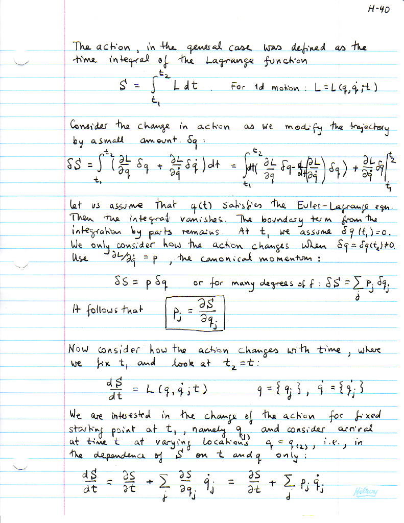
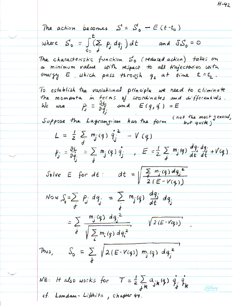
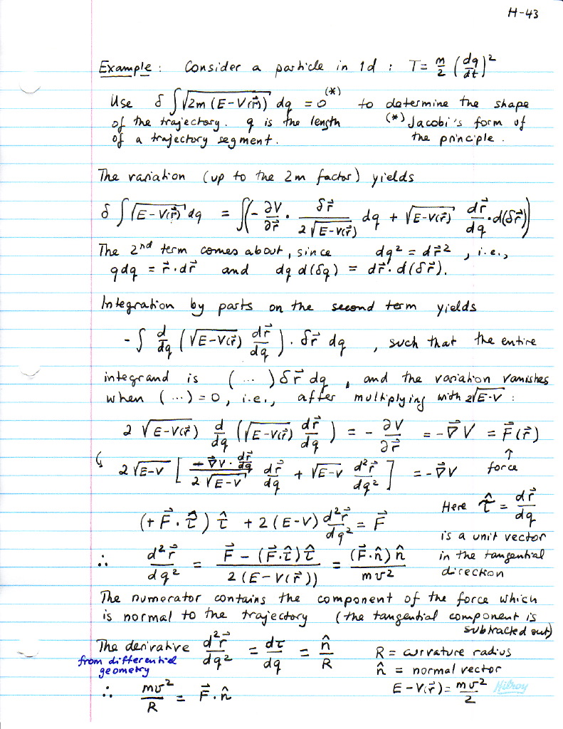
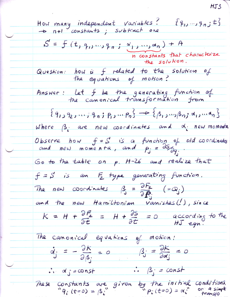
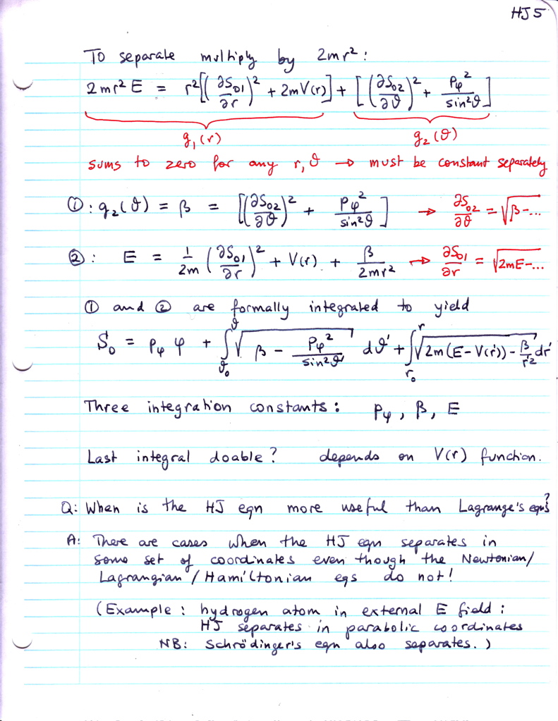
3.14 Hamilton-Jacobi mechanics HJ-2 Orbit shape Maupertuis principle Example
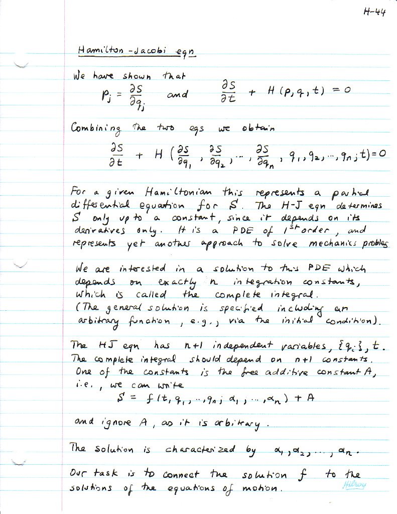
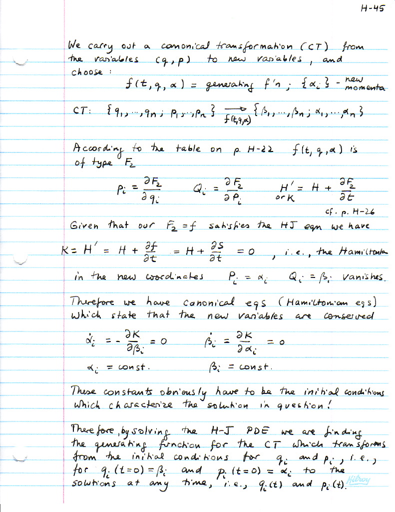
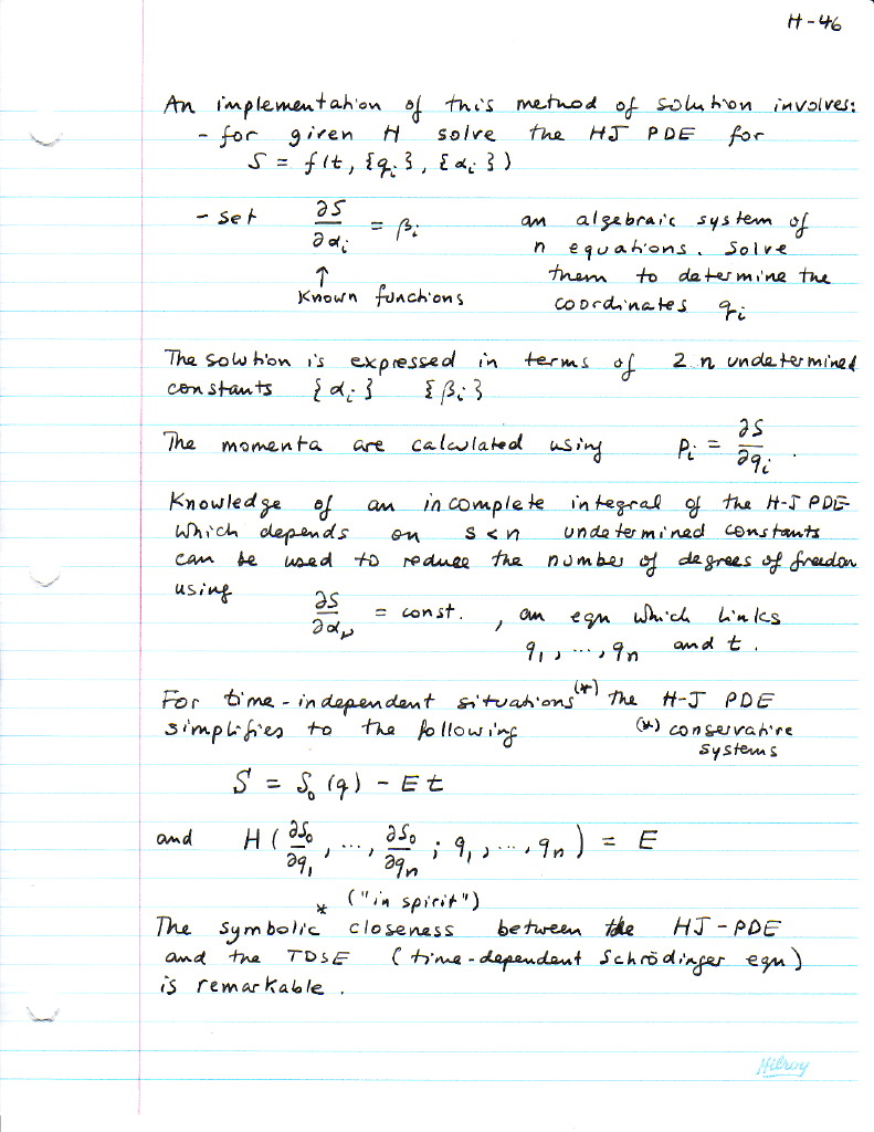
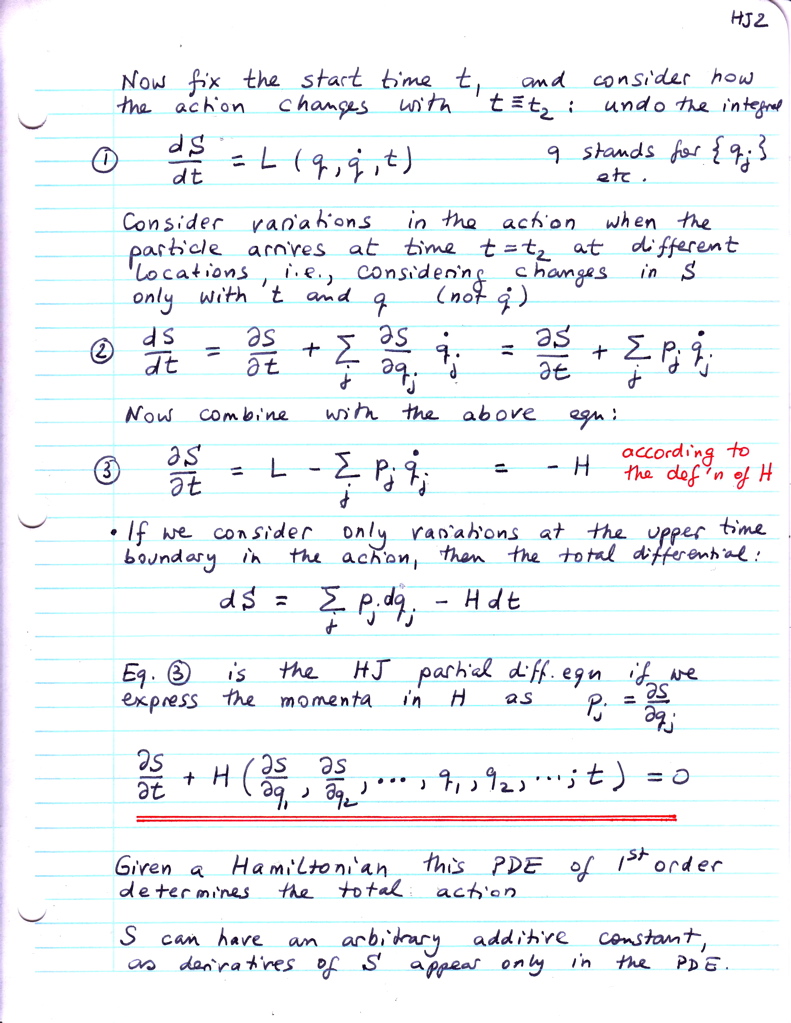
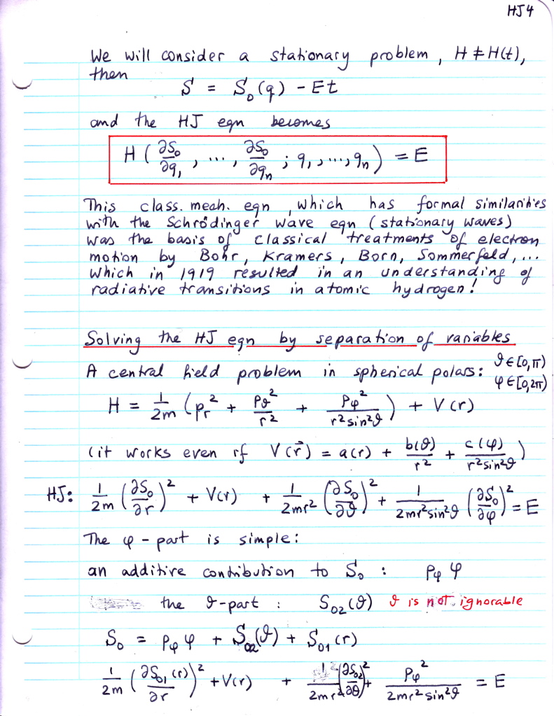
3.14 Hamilton-Jacobi equation HJE-2 HJE-3
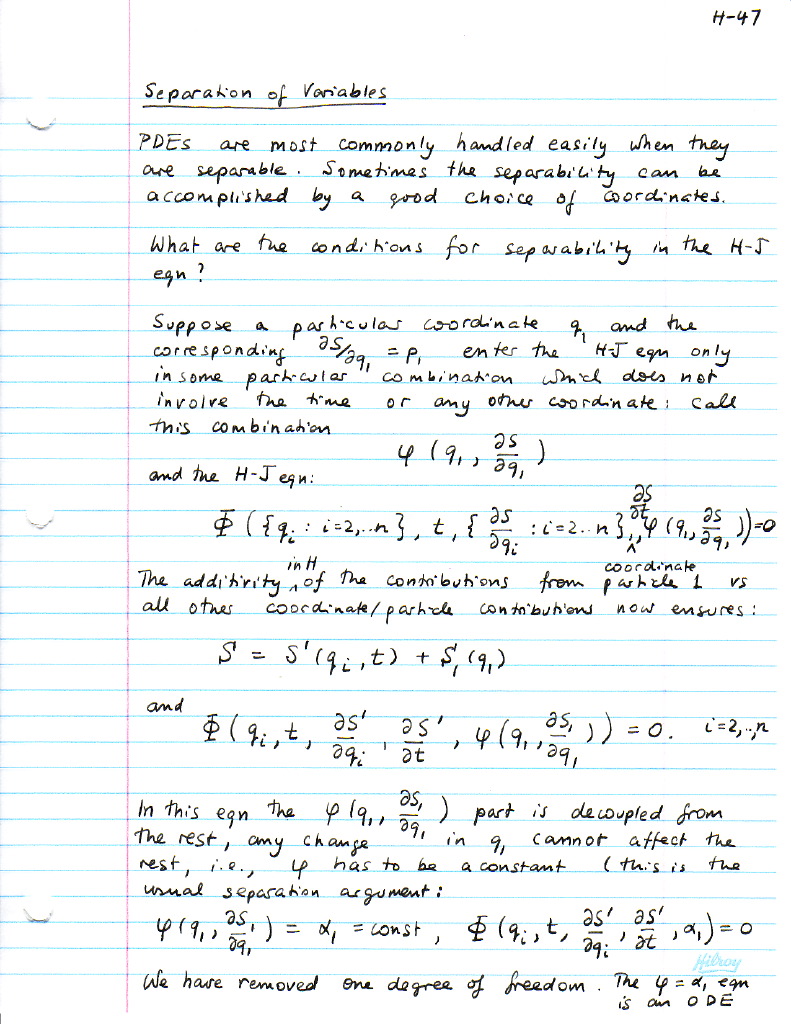
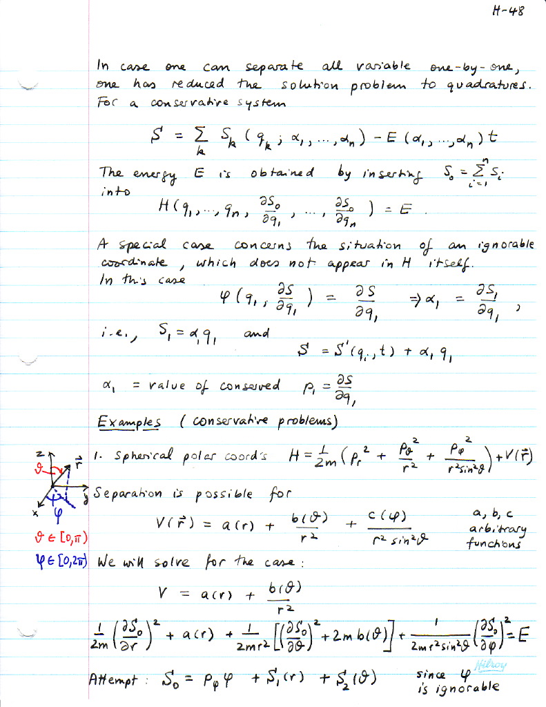
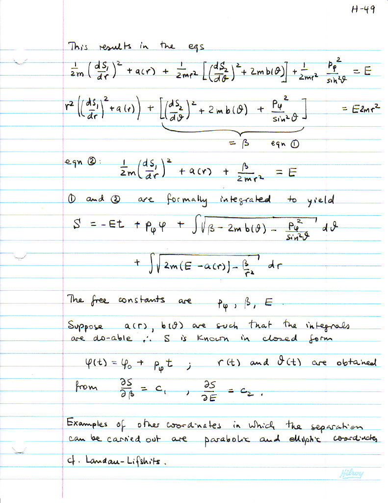
3.14 Separation of variables Example Ex-2
Notes for last class on the Hamilton-Jacobi equation to replace 3.14 ff: