Marko Horbatsch: marko@yorku.ca Petrie 230
Computational Methods for Physicists and Engineers (Symbolic Computation in Physics) PHYS 2030 3.0 webpage:
Fall 2005: Course notes, not just worksheets. Notes
An office hour with the teaching assistant/marker George Noble has been set up on Wednesdays, 4:30-5:30 pm, in Petrie 232A. First meeting time: Oct. 19.
Test 1 will be returned on Tuesday, Oct 27. The class average is 68.5%. A worksheet with the main parts to the solution can be downloaded here. Test1_2005.mws
Marking Scheme (2005):
Assignment 1 (10%) is due on Sept. 27
Assignment 2 (10%) is due on Oct. 18 (changed to Oct 27)
Class Test 1 (20%) is held on Oct. 20
Class Test 2 (30%) is held on Nov. 24
Assignment 3 (30%) is due on Dec 6
The class test on Nov 24 will be on Monte-Carlo integration. Class average: 71%, grades from 28 to 98.
Worksheet for MC: page2p3.mws
Matlab script for MC: page2p3.m
Assignment 3: The following problem is to be solved in two ways: (a) using Matlab or Maple's built-in ODE integrator; (b) using a second-order recursion of your own design (following our approach to the Kepler motion problem).
Consider two concentric cylinders, the inner with radius 1, the outer with radius 10. These are charged to a potential difference, such that an electron starting at the inner radius will accelerate towards the outer radius. In addition a homogeneous magnetic field can be turned on which is aligned with the cylinder axis. The motion is assumed to be in a plane, thus confined to be between circles of radius 1 and 10 respectively. The force law in our special units is given below.
F(x,y,v_x,v_y) = q (E(x,y) + (v_x,v_y,0) cross (0,0,B) )
Here the electric field E has x and y components such that q*E for the electron points radially outward, and its magnitude falls like 1/r, where r=sqrt(x^2+y^2). (think about the radially diverging field lines, whose density indicates the field strength). First solve with B=0 to make sure the radial motion is obtained correctly. Then try values of B such that the particles do not hit the outer cylinder. In our units q=1,m=1.
The use of Matlab is encouraged through a bonus of 10% points (on a 100-scale).
Assignment 2: There are two parts. In the first one we use Maple's dsolve command to obtain a symbolic solution to an ODE, in the second we solve numerically.
Part 1: Consider the damped harmonic oscillator (as discussed in class, but choose your own values for the mass and spring constant). Demonstrate solutions for the position as a function of time in three regimes: underdamped, overdamped, critically damped. For this you'll make appropriate choices of the damping constant b. Comment why critical damping is desirable for a spring/shock absorber system, while overdamping is not. Also display a phase-space plot for the three solutions, and explain which way the time evolution follows on them by adding arrows (by hand) to the Maple plots.
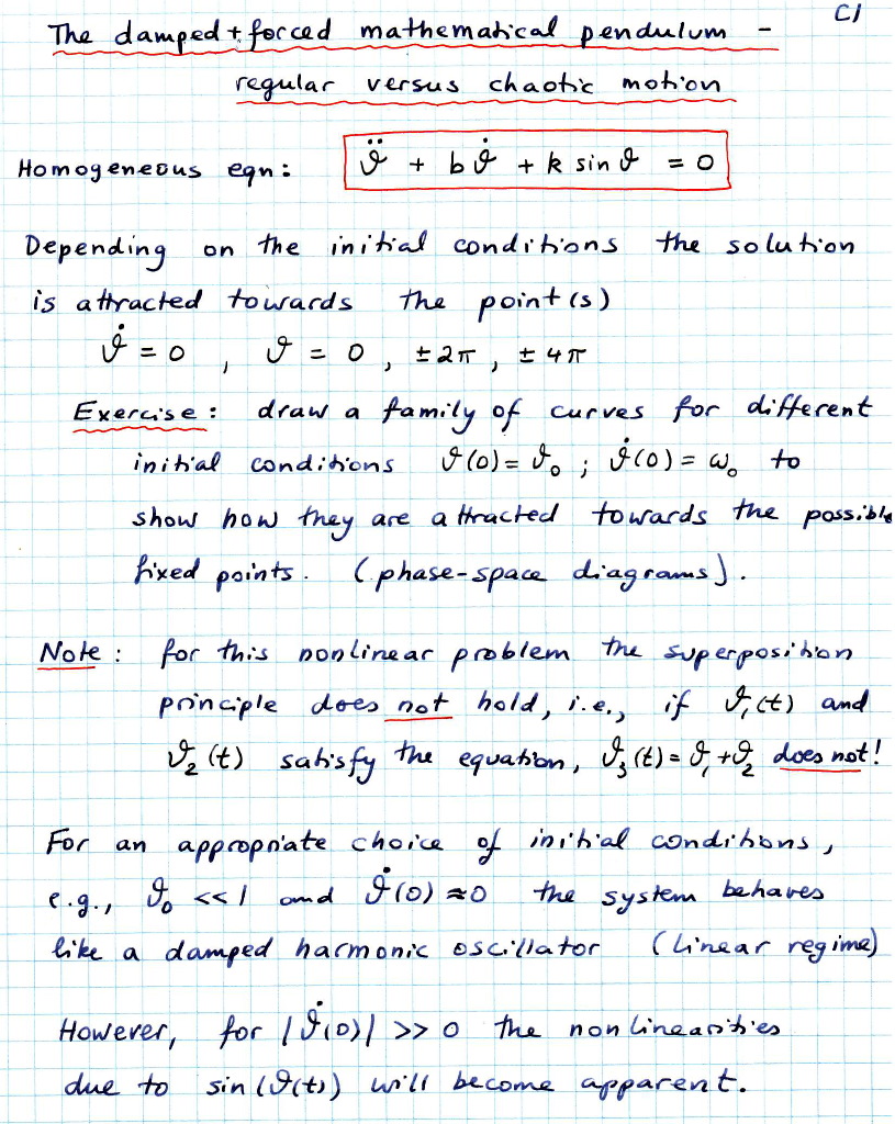
Part 2: Consider the mathematical pendulum (as discussed on p. 1.13 of the notes). The numerical solution in Maple is provided on page 1.15. Generate such solutions for damping constants B small enough to be in the underdamped regime. Obtain two types of solution, one in which the pendulum starts near the top with no initial rotation, and one where it has some angular velocity added. Comment on the meaning of the plots for theta(t), where theta is the angle of the pendulum arm with respect to the vertical. Also construct phase space diagrams [theta(t) versus w(t) parametrically, where w(t) is the angular velocity]. In you description of the motion pay attention to the fact that in a harmonic oscillator the oscillation frequency is independent of the intial amplitude. In the damped pendulum the frequency changes as the amplitude decreases. Demonstrate this point clearly using graphs.
Assignment 1: Go to lecture notes In1.1 to In1.3. For the problem of the circular rocket motion (which is solved there) complete the following graphs and explain them:
(1) the angular velocity w(t) for the time periods when the engine fires (0-10 seconds), as well as 10 seconds after that (10-20 seconds) when the engine has run out of fuel; superimpose the graphs using the display command from the plots package.
(2) for the same time periods, i.e., combined 0..20 seconds display the angle (in radians) as a function of time, theta(t).
(3) Using the angle theta(t) construct expressions for the Cartesian coordinates x(t) and y(t) in a reference frame that has the centre of the circle at its origin. Graph x(t) and y(t) on a single graph for the time t=0..20 seconds.
(4) Go to lecture notes In2.1-In2.2: Modify the maple code so that the object rolling down the incline is a sphere (not a cylinder). Compare the two solutions and provide a physical reason for the different answers.
Worksheet for Sept 13, 2005 (Tuesday class) Sept132005.mws
Worksheet for Sept 20, 2005 (Tuesday class) Sept202005.mws
Worksheet for Sept 27, 2005 (Tuesday class) Sept272005.mws
2 Worksheets for Oct 18, 2005 (Tuesday class) Oct182005.mws ; and CubicOscillator.mws
Worksheet for Oct 25, 2005 (Tuesday class) Oct252005.mws
Worksheet for Nov 8, 2005 (Tuesday class) Nov82005.mws
Worksheets for Nov 15, 2005 (Tuesday class) ExpUncertainty.mws ; and page2p4.mws ; and for matlab: page2p4.doc ; MI_Cone.m .
Worksheet for Nov 22, 2005 (Tuesday class) page2p5.mws . It includes an added part there the standard deviation of the mean is calculated by sampling the square of the measurement function. Matlab script that performs one potential energy evaluation with deviation based on sampling the square of the measurement function: PE_Sphere.m .
Worksheet for Nov29, 2005 (Tuesday class) EV.mws.
Class time: in contrast to previous years the class is split into one 2-hour session in a lecture hall (you can bring your laptop with maple and/or matlab if you like), and a 1-hour practice session in a PC lab with about 35 stations (team up if necessary, first-come first-served). The lectures will be held Tuesdays (9:40-11:20) in Curtis 110, the practice sessions Thursdays 10:30-11:20 in Steacie 021. The basement of the Steacie (Science Library) Building is a maze; there are numerous signs on the walls with arrows pointing you in the right direction.
Note: ALL STUDENTS SHOULD HAVE AN ACTIVE ACADLABS ACCOUNT when attending the first class, so that they can access the computers in the teaching lab Steacie 021. This also allows to use the computers in PSE 226 (Jupiter lab), and in the Commons (parking structure II).
SOFTWARE We will be using maple 9.5 and matlab. Versions maple8, maple9 or maple10 will work as well. We begin with maple, and an option to purchase it at a reduced cost compared to the UoT bookstore price is available further below. Please use ClassicWorksheet Maple9.5 from the ACADLABS server, I prefer it over the "new" Maple9 interface, and will be more efficient in assisting you. The two interfaces produce different worksheet files, I prefer the *.mws classic files.
UPDATED FOR 2005:
TO PURCHASE Student Maple9 for a special price (which is a deal maplesoft made for students of registered courses), use the following code: AD05061C on https://webstore.maplesoft.com/ The maplesoft page for the course is: http://www.maplesoft.com/academic/adoptioncenter/adoptioncenter_coursedetail.aspx?EID=37
There is no special deal for MATLAB. A student version can be purchased at University of Toronto bookstore, or directly on the internet from www.mathworks.com
TEXTBOOK(S) There is no textbook per se in this course. The course's main focus is to learn how to use Maple (and Matlab) to solve problems. Learning the programming environments will come as an aside. For the physics parts, and for some programming advice you will have my course notes (linked on this page). For Maple there are two reasonable guides linked as pdf's on this page, one is introductory, the other goes as far as you'll need in this course. I have also ordered two books for those who wish to have independent guides to the programming environments. These books are optional. I recommend for Maple: M.Abell&J.Braselton Maple by Example; for Matlab there is (the more expensive) D.Hanselman&B.Littlefield Mastering Matlab7. I have also asked UniText (across Campus on Keele) to order a cheaper alternative for Matlab, S.R.Otto&J.P.Denier An introduction to programming and numerical methods in MATLAB. Both Matlab books are useful and non-overlapping. The engineering students (for whom Matlab eventually will become more important than Maple) will benefit from both. The Otto&Denier was put on 1-day reserve in the library.
Professionalism and Punctuality This course is taught partly in a PC lab. If you come late to the lab, it is not only unprofessional, it disrupts the work of others, and sets you back more so than in regular lecture classes (where you can try to make up for missed material by reading up on it). Please do not come late, leave yourself room for traffic delays, etc. - you and your classmates will be the foremost beneficiaries. I will open the door to 021 Steacie on Thursdays a few minutes before 10:30 am, so that there will be time for the 35 stations to be activated.
Course Philosophy:
This course uses the Maple and later Matlab programs to deepen the physics understanding of topics encountered in first-year physics, and to explore the field of computational physics. Maple provides access to symbolic computation, graphing, algorithms and data structures. For this reason the course not only serves to deepen the understanding of physics and mathematics, but provides computational skills critical for any scientific career. We have developed many worksheets in the Computational Physics using Maple project; the course uses a small fraction of them, and leaves many pathways for further study all the way to graduate school.
Symbolic computing can cover only a part of a scientist or engineer's computing needs. Matlab represents an integrated computing/graphing environment that is up to 100 times faster in the computational domain than Maple. In the final quarter (or third) of the course we will solve some computationally intensive problems in this environment.
The teaching assistant for the course, George Noble, will hold an office hour at a time and location to be announced. Some guidelines for preparing assignments are given here Guidelines.doc.
Maple literature in pdf: Learning Guide; Programming Guide
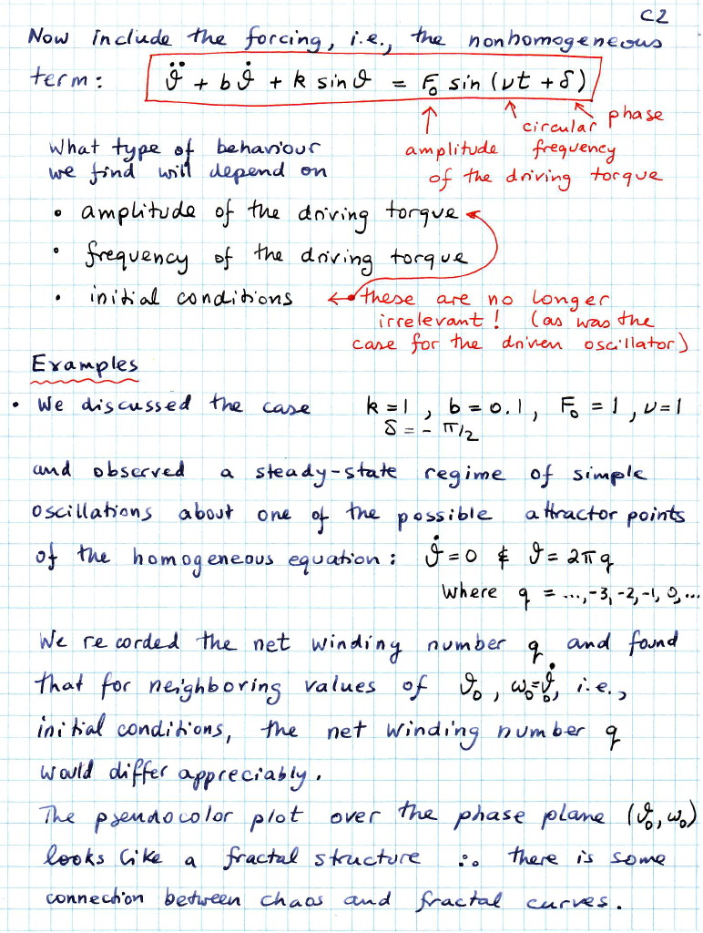
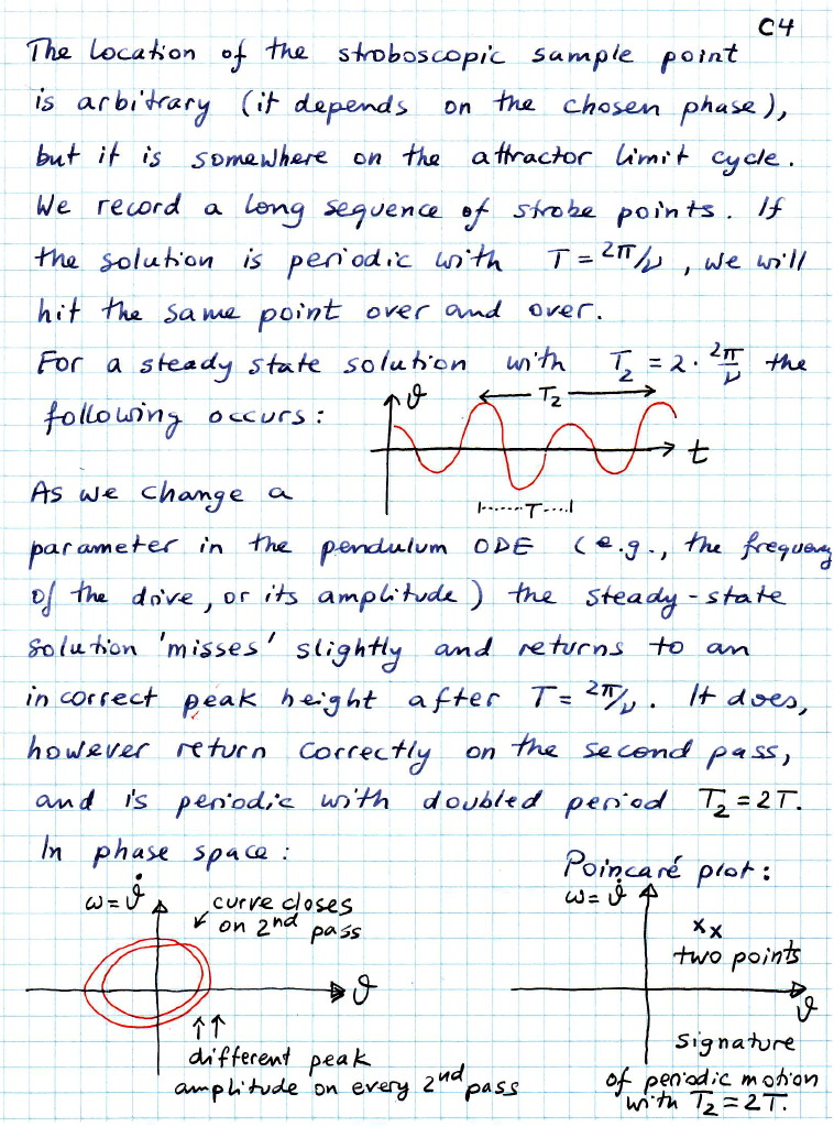
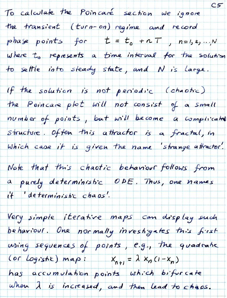
Notes on chaos in the driven pendulum:
Chaos1; Chaos2; Chaos3; Chaos4; Chaos5.
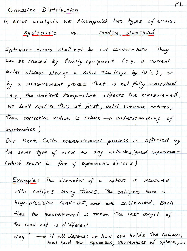
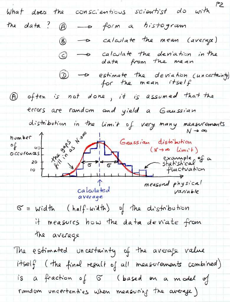
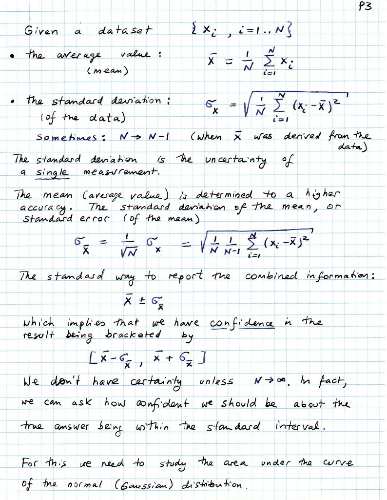
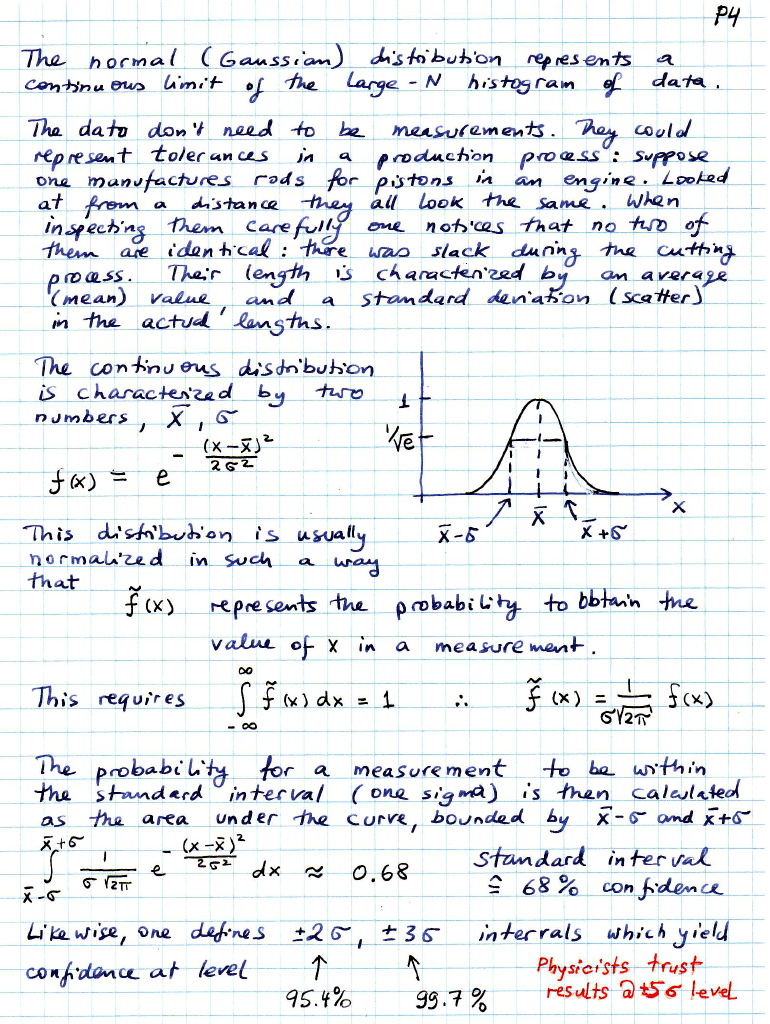
Notes on probability (the normal or the Gaussian distribution):
Some students asked me the question: "How do we input data into Maple from a datafile, e.g., from Excel?". Here is the answer that works in the windows or macintosh environment to read and write ASCII files, and also to do a linefit in maple in-between. IO.mws. The datafile from which to read is here: datafile.
My own Maple tutorial can be viewed here as HTML, and downloaded here as a Maple worksheet. The HTML is readable by any (recent-version) browser, but you can only look at it. The Maple worksheet is only useful if you access Maple, otherwise it is useless. This is the material that you will be able to use for reference during tests. If your browser shows a page full of goobledigook after you press the Maple link, proceed to save the file, using the suggested Reference.mws name, then open the file with Maple 9 (Classic Mode), or Maple 8 or Maple 7.