An internet resource developed by
Christopher D. Green
York University, Toronto, Ontario
ISSN 1492-3173
(Return to index)
STATISTICAL METHODS FOR RESEARCH WORKERS
By Ronald A. Fisher (1925)
Posted March 2000
III
DISTRIBUTIONS
11. The idea of an infinite population distributed in a frequency distribution in respect of one or more characters is fundamental to all statistical work. From a limited experience, for example, of individuals of a species, or of the weather of a locality, we may obtain some idea of the infinite hypothetical population from which our sample is drawn, and so of the probable nature of future samples to which our conclusions are to be applied. If a second sample belies this expectation we infer that it is, in the language of statistics, drawn from a different population; that the treatment to which the second sample of organisms had been exposed did in fact make a material difference, or that the climate (or the methods of measuring it) had materially altered. Critical tests of this kind may be called tests of significance, and when such tests are available we may discover whether a second sample is or is not significantly different from the first.
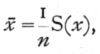
A statistic is a value calculated from an observed sample with a view to characterising the population [p. 44] from which it is drawn. For example, the mean of a number of observations x1, x2, . . . xn, is given by the equation
![]()
where S stands for summation over the whole sample, and n for the number of observations. Such statistics are of course variable from sample to sample, and the idea of a frequency distribution is applied with especial value to the variation of such statistics. If we know exactly how the original population was distributed it is theoretically possible, though often a matter of great mathematical difficulty, to calculate how any statistic derived from a sample of given size will be distributed. The utility of any particular statistic, and the nature of its distribution, both depend on the original distribution, and appropriate and exact methods have been worked out for only a few cases. The application of these cases is greatly extended by the fact that the distribution of many statistics tends to the normal form as the size of the sample is increased. For this reason it is customary to assume that such statistics are normally distributed, and to limit consideration of their variability to calculations of the standard error or probable error.
In the present chapter we shall give some account of three principal distributions -- (i.) the normal distribution, (ii.) the Poisson Series, (iii.) the binomial distribution. It is important to have a general knowledge of these three distributions, the mathematical formulæ by which they are represented, the experimental [p. 45] conditions upon which they occur, and the statistical methods of recognising their occurrence. On the latter topic we shall be led to some extent to anticipate methods developed more systematically in Chaps. IV. and V.
12. The Normal Distribution
A variate is said to be normally distributed when it takes all values from -[infinity], to +[infinity] , with frequencies given by a definite mathematical law, namely, that the logarithm of the frequency at any distance x from the centre of the distribution is less than the logarithm of the frequency at the centre by a quantity proportional to x2. The distribution is therefore symmetrical, with the greatest frequency at the centre; although the variation is unlimited, the frequency falls off to exceedingly small values at any considerable distance from the centre, since a large negative logarithm corresponds to a very small number. Fig. 6B represents a normal curve of distribution. The frequency [p. 46] in any infinitesimal range dx may be written as
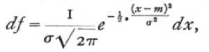
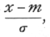
where x-m is the distance of the observation, x, from the centre of the distribution, m; and s, called the standard deviation, measures in the same units the extent to which the individual values are scattered. Geometrically s is the distance, on either side of the centre, of the steepest points, or points of inflexion of the curve (Fig. 4).
In practical applications we do not so often want to know the frequency at any distance from the centre as the total frequency beyond that distance; this is represented by the area of the tail of the curve cut off at any point. Tables of this total frequency, or probability integral, have been constructed from which, for any value of
we can find what fraction of the total population has a larger deviation; or, in other words, what is the probability that a value so distributed, chosen at random, shall exceed a given deviation. Tables I. and II. have been constructed to show the deviations corresponding to different values of this probability. The rapidity with which the probability falls off as the deviation increases is well shown in these tables. A deviation exceeding the standard deviation occurs about once in three trials. Twice the standard deviation is exceeded only about once in 22 trials, thrice the standard deviation only once in 370 trials, while Table II. shows that to exceed the standard deviation sixfold would need [p. 47] nearly a thousand million trials. The value for which P =·.05, or 1 in 20, is 1.96 or nearly 2 ; it is convenient to take this point as a limit in judging whether a deviation is to be considered significant or not. Deviations exceeding twice the standard deviation are thus formally regarded as significant. Using this criterion, we should be led to follow up a negative result only once in 22 trials, even if the statistics are the only guide available. Small effects would still escape notice if the data were insufficiently numerous to bring them out, hut no lowering of the standard of significance would meet this difficulty.
Some little confusion is sometimes introduced by the fact that in some cases we wish to know the probability that the deviation, known to be positive, shall exceed an observed value, whereas in other cases the probability required is that a deviation, which is equally frequently positive and negative, shall exceed an observed value; the latter probability is always half the former. For example, Table I. shows that the normal deviate falls outside the range [plus or minus]1.598193 in 10 per cent of cases, and consequently that it exceeds +1.598193 in 5 per cent of cases.
The value of the deviation beyond which half the observations lie is called the quartile distance, and bears to the standard deviation the ratio .67449.·It is therefore a common practice to calculate the standard error and then, multiplying it by this factor, to obtain the probable error. The probable error is thus about two-thirds of the standard error, and as a test of significance a deviation of three times [p. 48] the probable error is effectively equivalent to one of twice the standard error. The common use of the probable error is its only recommendation ; when any critical test is required the deviation must be expressed in terms of the standard error in using the probability integral table.
13. Fitting the Normal Distribution
From a sample of n individuals of a normal population the mean and standard deviation of the population may be estimated by means of two easily calculated statistics. The best estimate of m is x where
while for the best estimate of s, we calculate s from
![]()
these two statistics are calculated from the first two moments (see Appendix, p. 74) of the sample, and are specially related to the normal distribution, in that they summarise the whole of the information which the sample provides as to the distribution from which it was drawn, provided the latter was normal. Fitting by moments has also been widely applied to skew (asymmetrical) curves, and others which are not normal; but such curves have not the peculiar properties which make the first two moments especially appropriate, and where the curves differ widely from the normal form the above two statistics may be of little or no use.
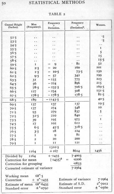
Ex. 2. Fitting a normal distribution to a large [p. 49] sample. -- In calculating the statistics from a large sample it is not necessary to calculate individually the squares of the deviations from the mean of each measurement. The measurements are grouped together in equal intervals of the variate, and the whole of the calculation may be carried out rapidly as shown in Table 2, where the distribution of the stature of 1164 men is analysed.
The first column shows the central height in inches of each group, followed by the corresponding frequencies. A central group (68.5") is chosen as "working mean." To form the next column the frequencies are multiplied by 1, 2, 3, etc., according to their distance from the working mean; this process being repeated to form the fourth column, which is summed from top to bottom in a single operation; in the third column, however, the upper portion, representing negative deviations, is summed separately, and subtracted from the sum of the lower portion. The difference, in this case positive, shows that the whole sample of 1164 individuals has in all 167 inches more than if every individual were 68.5" in height. This balance divided by 1164 gives the amount by which the mean of the sample exceeds 68.5". The mean of the sample is therefore 68.6435". The sum of the fourth column is also divided by 1164, and gives an uncorrected estimate of the variance; two corrections are then applied -- one is for the fact that the working mean differs from the true mean, and consists in subtracting the square of the difference ; the second, which is Sheppard's correction for grouping, [p. 50] [table] [p. 51] allows for the fact that the process of grouping tends somewhat to exaggerate the variance, since in each group the values with deviations smaller than the central value will generally be more numerous than the values with deviations larger than the central value. Working in units of grouping, this correction is easily applied by subtracting a constant quantity 1/12 (=.0833) from the variance. From the variance so corrected the standard deviation is obtained by taking the square root. This process may be carried through as an exercise with the distribution of female statures given in the same table (p. 103).
Any interval may be used as a unit of grouping; and the whole calculation is carried through in such units, the final results being transformed into other units if required, just as we might wish to transform the mean and standard deviation from inches to centimetres by multiplying by the appropriate factor. It is advantageous that the units of grouping should be exact multiples of the units of measurement ; so that if the above sample had been measured to tenths of an inch, we might usefully have grouped them at intervals of 0.6" or 0.7".
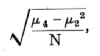
Regarded as estimates of the mean and standard deviation of a normal population of which the above is regarded as a sample, the values found are affected by errors of random sampling; that is, we should not expect a second sample to give us exactly the same values. The values for different (large) samples of the same size would, however, be distributed very accurately in normal distributions, so the accuracy of [p. 52] any one such estimate may be satisfactorily expressed by its standard error. These standard errors may be calculated from the standard deviation of the population, and in treating large samples we take our estimate of this standard deviation as the basis of the calculation. The formulæ for the standard errors of random sampling of estimates of the mean and standard deviation of a large normal sample are (as given in Appendix, p. 75)
![]()
and their numerical values have been appended to the quantities to which they refer. From these values it is seen that our sample shows significant aberration from any population whose mean lay outside the limits 68.48"-68.80", and it is therefore likely that the mean of the population from which it was drawn lay between these limits; similarly it is likely that its standard deviation lay between 2.59" and 2·81".
It may be asked, Is nothing lost by grouping? Grouping in effect replaces the actual data by fictitious data placed arbitrarily at the central values of the groups; evidently a very coarse grouping might be very misleading. It has been shown that as regards obtaining estimates of the parameters of a normal population, the loss of information caused by grouping is less than 1 per cent, provided the group interval does not exceed one quarter of the standard deviation ; the grouping of the above sample in whole inches is thus somewhat too coarse; the loss in the estimation of the [p. 53] standard deviation is 2.28 per cent, or about 27 observations out of 1164; the loss in the estimation of the mean is half as great. With suitable group intervals, however, little is lost by grouping, and much labour is saved.
Another way of regarding the loss of information involved in grouping is to consider how near the values obtained for the mean and standard deviation will be to the values obtained without grouping. From this point of view we may calculate a standard error of grouping, not to be confused with the standard error of random sampling which measures the deviation of the sample values from the population value. In grouping units, the standard error due to grouping of both the mean and the standard deviation is

or in this case 0085". For sufficiently fine grouping this should not exceed one-tenth of the standard error of random sampling.
In the above analysis of a large sample the estimate of the variance employed was
which differs from the formula given previously (p. 48) in that we have divided by n instead of by (n-1). In large samples the difference between these formulæ is small, and that using n may claim a theoretical advantage if we wish for an estimate to be used in conjunction with the estimate of the mean from the [p. 54] same sample, as in fitting a frequency curve to the data; otherwise it is best to use (n-1). In small samples the difference is still small compared to the probable error, but becomes important if a variance is estimated by averaging estimates from a number of small samples. Thus if a series of experiments are carried out each with six parallels and we have reason to believe that the variation is in all cases due to the operation of analogous causes, we may take the average of such quantities as
![]()
to obtain an unbiassed estimate of the variance, whereas we should under-estimate it were we to divide by 6.
14. Test of Departure from Normality
It is sometimes necessary to test whether an observed sample does or does not depart significantly from normality. For this purpose the third, and sometimes the fourth moment, is calculated; from each of these it is possible to calculate a quantity, g, which is zero for a normal distribution, and is distributed normally about zero for large samples; the standard error being calculable from the size of the sample.
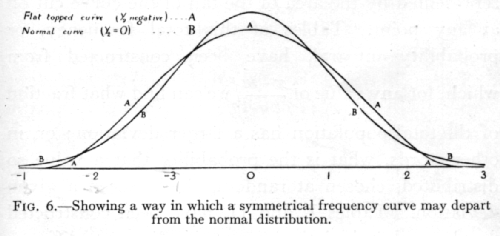
The quantity g1, which is calculated from the third moment, is essentially a measure of asymmetry; it is equal to [plus or minus][sqrt]b1, of Pearson's notation; g2(=b2-3), calculated from the fourth moment, measures a symmetrical type of departure from the normal form, [p. 55] by which the apex and the two tails of the curve are increased at the expense of the intermediate portion, or, when g2, is negative, the top and tails are depleted and the shoulders filled out, making a relatively flat-topped curve. (See Fig. 6, p. 45·)
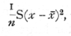
Ex. 3. Use of higher moments to test normality. -- Departures from normal form, unless very strongly marked, can only be detected in large samples; we give an example (Table 3) of the calculation for 65 values of the yearly rainfall at Rothamsted; the process of calculation is similar to that of finding the mean and standard deviation, but it is carried two stages further, in the calculation of the 3rd and 4th moments. The formulæ by which the two corrections are applied to the moments are gathered in an appendix, p. 74· For the moments we obtain
![]()
whence are calculated
![]()
For samples from a normal distribution the standard errors of g1 and g2 are [sqrt]6/n and [sqrt]24/n, of which the numerical values are given. It will be seen that g1, exceeds its standard error, but g2, is quite insignificant; since g1, is positive it appears that there may be some asymmetry of the distribution in the sense that moderately dry and very wet years are respectively more frequent than moderately wet and very dry years. [p. 56]
15. Discontinuous Distributions
Frequently a variable is not able to take all possible values, but is confined to a particular series of values, such as the whole numbers. This is obvious when the variable is a frequency, obtained by counting, such as the number of cells on a square of a hæmocytometer, [p. 57] or the number of colonies on a plate of culture medium. The normal distribution is the most important of the continuous distributions; but among discontinuous distributions the Poisson Series is of the first importance. If a number can take the values 0, 1, 2, . . ., x, . . ., and the frequency with which the values occur are given by the series
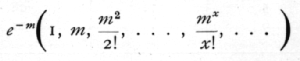
(where x! stands for "factorial x" =x(x-1)(x-2) ... 1), then the number is distributed in the Poisson Series. Whereas the normal curve has two unknown parameters, m and s, the Poisson Series has only one. This value may be estimated from a series of observations, by taking their mean, the mean being a statistic as appropriate to the Poisson Series as it is to the normal curve. It may be shown theoretically that if the probability of an event is exceedingly small, but a sufficiently large number of independent cases are taken to obtain a number of occurrences, then this number will be distributed in the Poisson Series. For example, the chance of a man being killed by horse-kick on any one day is exceedingly small, but if an army corps of men are exposed to this risk for a year, a certain number of them will often be killed in this way. The following data (Bortkewitch's data) were obtained from the records of ten army corps for twenty years: [p. 58]
The average, m, is .61, and using this value the numbers calculated agree excellently with those observed.
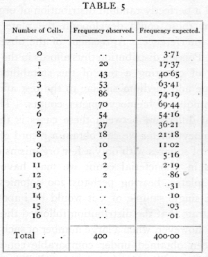
The importance of the Poisson Series in biological research was first brought out in connexion with the accuracy of counting with a hæmocytometer. It was shown that when the technique of the counting process was effectively perfect, the number of cells on each square should be theoretically distributed in a Poisson Series; it was further shown that this distribution was, in favourable circumstances, actually realised in practice. Thus the table on page 59 (Student's data) shows the distribution of yeast cells in the 400 squares into which one square millimetre was divided.
The total number of cells counted is 1872, and the mean number is therefore 4.68. The expected frequencies calculated from this mean agree well with those observed. The methods of resting the agreement are explained in Chapter IV.
When a number is the sum of several components each of which is independently distributed in a Poisson [p. 59] Series, then the total number is also so distributed. Thus the total count of 1872 cells may be regarded as a single sample of a series, for which m is not far from 1872. For such large values of m the distribution of numbers approximates closely to the normal form, in such a way that the variance is equal to m; we may therefore attach to the number counted, 1872, the standard error [plus of minus][sqrt]1872 = [plus or minus]43.26, to represent the standard error of random sampling of such a count. The density of cells in the original suspension is therefore estimated with a standard error of 2.31 per cent. If, for instance, a second sample differed by 7 per cent, the technique of sampling would be suspect. [p. 60]
16. Small Samples of a Poisson Series
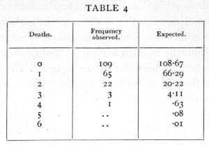
Exactly the same principles as govern the accuracy of a hæmocytometer count would also govern a count of bacterial or fungal colonies in estimating the numbers of those organisms by the dilution method, if it could be assumed that the technique of dilution afforded a perfectly random distribution of organisms, and that these could develop on the plate without mutual interference. Agreement of the observations with the Poisson distribution thus affords in the dilution method of counting a test of the suitability of the technique and medium similar to the test afforded of the technique of hæmocytometer counts. The great practical difference between these cases is that from the hæmocytometer we can obtain a record of a large number of squares with only a few organisms on each, whereas in a bacterial count we may have only 5 parallel plates, bearing perhaps 200 colonies apiece. From a single sample of 5 it would be impossible to demonstrate that the distribution followed the Poisson Series; however, when a large number of such samples have been obtained under comparable conditions, it is possible to utilise the fact that for all Poisson Series the variance is numerically equal to the mean.
For each set of parallel plates with x1, x2, . . ., xn, colonies respectively, taking the mean x[bar], an index of dispersion may be calculated by the formula
![]() [p. 61]
[p. 61]
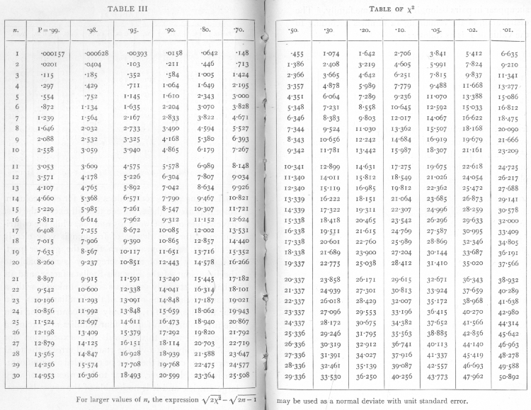
It has been shown that for true samples of a Poisson Series, χ2 calculated in this way will be distributed in a known manner; Table III. (p. 98) shows the principal values of χ2 for this distribution; entering the table take n equal to one less than the number of parallel plates. For small samples the permissible range of variation of χ2 is wide; thus for five plates with n=4, χ2 will be less than 1.064 in 10 per cent of cases, while the highest 10 per cent will exceed 7.779; a single sample of 5 thus gives us little information; but if we have 50 or 100 such samples, we are in a position to verify with accuracy if the expected distribution is obtained.
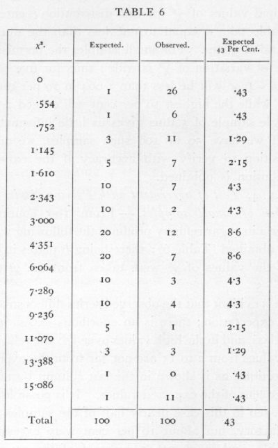
Ex. 4· Test of agreement with a Poisson Series of a number of small samples. -- From 100 counts of bacteria in sugar refinery products the following values were obtained (Table 6); there being 6 plates in each case, the values of χ2 were taken from the χ2 table for n =5.
It is evident that the observed series differs strongly from expectation; there is an enormous excess in the first class, and in the high values over 15; the relatively few values from 2 to 15 are not far from the expected proportions, as is shown in the last column by taking 43 per cent of the expected values. It is possible then that even in this case nearly half of the samples were satisfactory, but about 10 per cent were excessively variable, and in about 45 per cent of the cases the variability was abnormally depressed.
It is often desirable to test if the variability is of the right magnitude when we have not accumulated [p. 62] a large number of counts, all with the same number of parallel plates, but where a certain number of counts are available with various numbers of parallels. In this case we cannot indeed verify the theoretical distribution with any exactitude, but can test whether [p. 63] or not the general level of variability conforms with expectation. The sum of a number of independent values of χ2 is itself distributed in the manner shown in the table of χ2, provided we take for n the number S(n), calculated by adding the several values of n for the separate experiments. Thus for six sets of 4 plates each the total value of χ2 was found to be 1385, the corresponding value of n is 6x3=18, and the χ2 table shows that for n=18 the value 13.85 is exceeded in between 70 and 80 per cent of cases ; it is therefore not an abnormal value to obtain. In another case the following values were obtained:
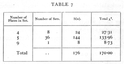
We have therefore to test if χ2=170 is an unreasonably small or great value for n=176· The χ2 table has not been calculated beyond n=30, but for higher values we make use of the fact that the distribution of χ2 becomes nearly normal. A good approximation is given by assuming that ([sqrt]2χ2 - [sqrt]2n-1 is normally distributed about zero with unit standard deviation. If this quantity is materially greater than 2, the value of χ2 is not in accordance with expectation. In the example before us [p. 64]
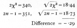
The set of 45 counts thus shows variability between parallel plates, very close to that to be expected theoretically. The internal evidence thus suggests that the technique was satisfactory.
17. Presence and Absence of Organisms in Samples
When the conditions of sampling justify the use of the Poisson Series, the number of samples containing 0, 1, 2, ... organisms is, as we have seen, connected by a calculable relation with the mean number of organisms in the sample. With motile organisms, or in other cases which do not allow of discrete colony formation, the mean number of organisms in the sample may be inferred from the proportion of fertile cultures, provided a single organism is capable of developing. If m is the mean number of organisms in the sample, the proportion of samples containing none, that is the proportion of sterile samples, is e-m, from which relation we can calculate, as in the following table, the mean number of organisms corresponding to 10 per cent, 20 per cent, etc., fertile samples:
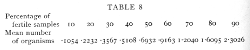
In connexion with the use of the above table it is worth noting that for a given number of samples [p. 65] tested the percentage is most accurately determined at 50 per cent, but for the minimum percentage error in the estimate of the number of organisms, nearly 60 per cent or 88 organisms per sample is most accurate. The Poisson Series also enables us to calculate what percentage of the fertile cultures obtained have been derived from a single organism, for the percentage of impure cultures, i.e. those derived from 2 or more organisms, can be calculated from the percentage of cultures which proved to be fertile. If e-m are sterile, me-m will be pure cultures, and the remainder impure. The following table gives representative values of the percentage of cultures which are fertile, and the percentage of fertile cultures which are impure:
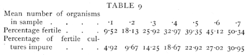
If it is desired that the cultures should be pure with high probability, a sufficiently low concentration must be used to render at least nine-tenths of the samples sterile.
18. The Binomial Distribution
The binomial distribution is well known as the first example of a theoretical distribution to be established. It was found by Bernoulli, about the beginning of the eighteenth century, that if the probability of an event occurring were p and the probability of it not occurring were q(=1-p), then if a random sample of n trials [p. 66] were taken, the frequencies with which the event occurred 0, 1, 2,..., n times were given by the expansion of the binomial
(q+p)n.
This rule is a particular case of a more general theorem dealing with cases in which not only a simple alternative is considered, but in which the event may happen in s ways with probabilities p1, p2 ..., ps; then it can be shown that the chance of a random sample of n giving a1, of the first kind, a2, of the second, ..., as of the last is
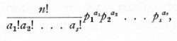
which is the general term in the multinomial expansion of
(p1+p2+...+ps)n.
Ex. 5· Binomial distribution given by dice records. -- In throwing a true die the chance of scoring more than 4 is 1/3, and if 12 dice are thrown together the number of dice scoring 5 or 6 should be distributed with frequencies given by the terms in the expansion of
(2/3 + 1/3)12
If, however, one or more of the dice were not true, but if all retained the same bias throughout the experiment, the frequencies should be given approximately by
(q+p)12,
where p is a fraction to be determined from the data. [p. 67] The following frequencies were observed (Weldon's data) in an experiment of 26,306 throws.
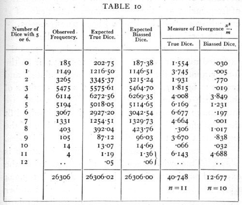
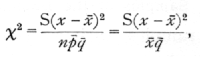
It is apparent that the observations are not compatible with the assumption that the dice were. unbiassed. With true dice we should expect more cases than have been observed of 0, 1, 2, 3, 4, and less cases than have been observed of 5, 6, ..., 11 dice scoring more than four. The same conclusion is more clearly brought out in the fifth column, which shows the values of the measure of divergence
![]()
where m is the expected value and x the difference [p. 68] between the expected and observed values. The aggregate of these values is χ2, which measures the deviation of the whole series from the expected series of frequencies, and the actual chance in this case of χ2 exceeding 40.75 if the dice had been true is .00003.
The total number of times in which a die showed 5 or 6 was 106,602, out of 315,672 trials, whereas the expected number with true dice is 105,224; from the former number, the value of p can be calculated, and proves to be .337,698,6, and hence the expectations of the fourth column were obtained. These values are much more close to the observed series, and indeed fit them satisfactorily, showing that the conditions of the experiment were really such as to give a binomial series.
The standard deviation of the binomial series is [sqrt]pqn. Thus with true dice and 315,672 trials the expected number of dice scoring more than 4 is 105,224 with standard error 264.9; the observed number exceeds expectation by 2378, or 5.20 times its standard error; this is the most sensitive test of the bias, and it may be legitimately applied, since for such large samples the binomial distribution closely approaches the normal. From the table of the probability integral it appears that a normal deviation only exceeds 5.2 times its standard error once in 5 million times.
The reason why this last test gives so much higher odds than the test for goodness of fit, is that the latter is testing for discrepancies of any kind, such, for example, as copying errors would introduce. The actual discrepancy is almost wholly due to a single item, namely, the value of p, and when that point [p. 69] is tested separately its significance is more clearly brought out.
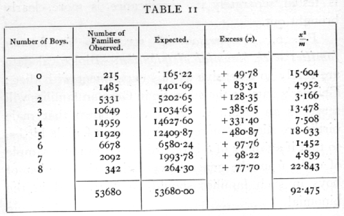
Ex. 6. Comparison of sex ratio in human families with the binomial distribution. -- Biological data are rarely so extensive as this experiment with dice; Geissler's data on the sex ratio in German families will serve as an example. It is well known that male births are slightly more numerous than female births, so that if a family of 8 is regarded as a random sample of eight from the general population, the number of boys in such families should be distributed in the binomial
(q+p)8,
where p is the proportion of boys. If, however, families differ not only by chance, but by a tendency on the part of some parents to produce males or females, then the distribution of the number of boys should show an excess of unequally divided families, and a deficiency of equally or nearly equally divided families. The data in Table 11 show that there is evidently such an excess of very unequally divided families.
The observed series differs from expectation markedly in two respects: one is the excess of unequally divided families; the other is the irregularity of the central values, showing an apparent bias in favour of even values. No biological reason is suggested for the latter discrepancy, which therefore detracts from the value of the data. The excess of the extreme types of family may be treated in more detail by [p. 70] comparing the observed with the expected variance. The expected variance, npq, calculated from the data is 1.998,28, while that calculated from the data is 2.067,42, showing an excess of .06914, or 3.46 per cent. The standard error of the variance is
where N is the number of samples, and m2 and m4, are the second and fourth moments of the theoretical distribution, namely,
![]()
so that
![]()
The approximate values of these two terms are 8 and -1 giving +7, the actual value being 6.98966. Hence the standard error of the variance is .01141; the discrepancy is over six times its standard error. [p. 71]
One possible cause of the excessive variation lies in the occurrence of multiple births, for it is known that children of the same birth tend to be of the same sex. The multiple births are not separated in these data, but an idea of the magnitude of this effect may be obtained from other data for the German Empire. These show about 12 twin births per thousand, of which 5/8 are of like sex and 3/8 of unlike, so that one-quarter of the twin births, 3 per thousand, may be regarded as "identical" in respect of sex. Six children per thousand would therefore probably belong to such "identical" twin births, the additional effect of triplets, etc., being small. Now with a population of identical twins it is easy to see that the theoretical variance is doubled; consequently, to raise the variance by 3.46 per cent we require that 3.46 per cent of the children should be "identical" twins; this is more than five times the general average, and although it is probable that the proportion of twins is higher in families of 8 than in the general population, we cannot reasonably ascribe more than a fraction of the excess variance to multiple births.
19. Small Samples of the Binomial Series
With small samples, such as ordinarily occur in experimental work, agreement with the binomial series cannot be tested with such precision from a single sample. It is, however, possible to verify that the variation is approximately what it should be, by calculating an index of dispersion similar to that used for the Poisson Series. [p. 72]
Ex. 7· The accuracy of estimates of infestation. -- The proportion of barley ears infected with goutfly may be ascertained by examining 100 ears, and counting the infected specimens; if this is done repeatedly, the numbers obtained, if the material is homogeneous, should be distributed in the binomial
(q+p)100,
where p is the proportion infested, and q the proportion free from infestation. The following are the data from 10 such observations made on the same plot (J. G. H. Frew's data):
16, 18, 11, 18, 21, 10, 20, 18, 17, 21. Mean 17.0·
Is the variability of these numbers ascribable to random sampling; i.e. Is the material apparently homogeneous? Such data differs from that to which the Poisson Series is appropriate, in that a fixed total of 100 is in each case divided into two classes, infected and not infected, so that in taking the variability of the infected series we are equally testing the variability of the series of numbers not infected. The modified form of χ2, the index of dispersion, appropriate to the binomial is
differing from the form appropriate to the Poisson Series in containing the divisor q[bar], or in this case, .83.· The value of χ2 is 9.22, which, as the χ2, table shows, is a perfectly reasonable value for n=9, one less than the number of values available. [p. 73]
Such a test of the single sample is, of course, far from conclusive, since χ2 may vary within wide limits. If, however, a number of such small samples are available, though drawn from plots of very different infestation, we can test, as with the Poisson Series, if the general trend of variability accords with the binomial distribution. Thus from 20 such plots the total χ2 is 193.64, while S(n) is 180. Testing as before (p. 63), we find
The difference being less than one, we conclude that the variance shows no sign of departure from that of the binomial distribution. The difference between the method appropriate for this case, in which the samples are small (10), but each value is derived from a considerable number (100) of observations, and that appropriate for the sex distribution in families of 8, where we had many families, each of only 8 observations, lies in the omission of the term
npq(1-6pq)
in calculating the standard error of the variance. When n is 100 this term is very small compared to 2n2p2q2, and in general the χ2 method is highly accurate if the number in all the observational categories is as high as 10. [p. 74]
APPENDIX OF TECHNICAL NOTATION AND FORMULÆ
A. Definition of moments of sample.
The following statistics are known as the first four moments of the variate x; the first moment is the mean
the second and higher moments are the mean values of the second and higher powers of the deviations from the mean
B. Moments of theoretical distribution in terms of parameters.
[p. 75]
C. Variance of moments derived from samples of N.
D. Corrections in calculating moments.
(a) Correction for mean, if v' is the moment about the working mean, and v the corresponding value corrected to the true mean:
v2 = v'2 - v'12,
v3 = v'3 - 3v'1v'2 + 2v'13,
v4 = v'4 - 4v'1v'3 + 6v'12v'2 - 3v'14.
(b) Correction for grouping, if v is the estimate uncorrected for grouping, and m the corresponding estimate corrected:
m
1 = v2 - 1/12,m
2 = v3,m
3 = v4 -1/2m2 - 1/80. [p. 76]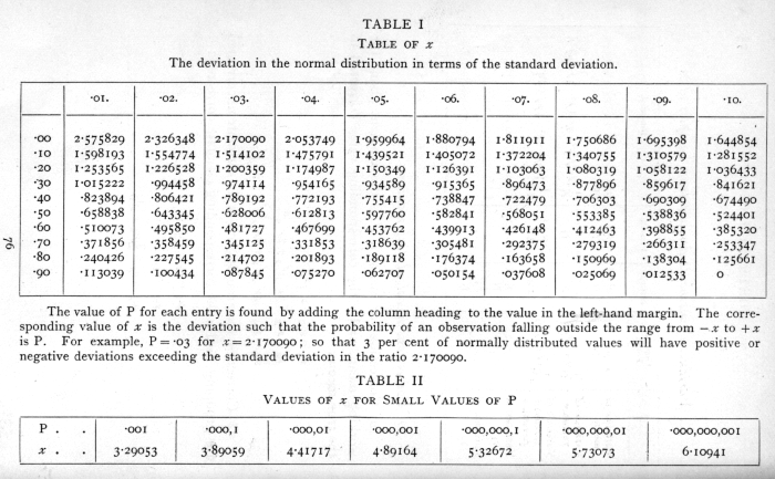