An internet resource developed by
Christopher D. Green
York University, Toronto, Ontario
ISSN 1492-3173
(Return to index)
By Ronald A. Fisher (1925)
Posted April 2000
VI
THE CORRELATION COEFFICIENT
30. No quantity is more characteristic of modern statistical work than the correlation coefficient, and no method has been applied successfully to such various data as the method of correlation. Observational data in particular, in cases where we can observe the occurrence of various possible contributory causes of a phenomenon, but cannot control them, has been given by its means an altogether new importance. In experimental work proper its position is much less central; it will be found useful in the exploratory stages of an enquiry, as when two factors which had been thought independent appear to be associated in their occurrence; but it is seldom, with controlled experimental conditions, that it is desired to express our conclusion in the form of a correlation coefficient.
One of the earliest and most striking successes of the method of correlation was in the biometrical study of inheritance. At a time when nothing was known of the mechanism of inheritance, or of the structure of the germinal material, it was possible by this method to demonstrate the existence of inheritance, and to [p. 139] "measure its intensity"; and this in an organism in which experimental breeding could not be practised, namely, Man. By comparison of the results obtained from the physical measurements in man with those obtained from other organisms, it was established that man's nature is not less governed by heredity than that of the rest of the animate world. The scope of the analogy was further widened by demonstrating that correlation coefficients of the same magnitude were obtained for the mental and moral qualities in man as for the physical measurements.
These results are still of fundamental importance, for not only is inheritance in man still incapable of experimental study, and existing methods of mental testing are still unable to analyse the mental disposition, but even with organisms suitable for experiment and measurement, it is only in the most favourable cases that the several factors causing fluctuating variability can be resolved, and their effects studied, by Mendelian methods. Such fluctuating variability, with an approximately normal distribution, is characteristic of the majority of the useful qualities of domestic plants and animals; and although there is strong reason to think that inheritance in such cases is ultimately Mendelian, the biometrical method of study is at present alone capable of holding out hopes of immediate progress.
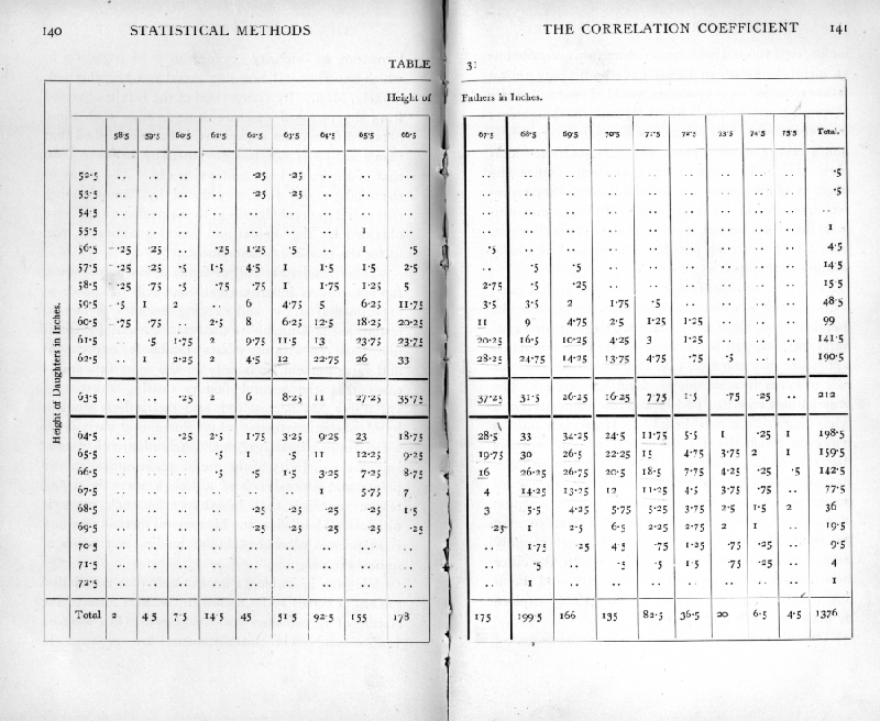
We give in Table 31 an example of a correlation table. It consists of a record in compact form of the stature of 1376 fathers and daughters. (Pearson and Lee's data.) The measurements are grouped in [p. 140-141] [table] [p. 142] inches, and those whose measurement was recorded as an integral number of inches have been split; thus a father recorded as of 67 inches would appear as 1/2 under 66.5 and 1/2 under 67.5. Similarly with the daughters; in consequence, when both measurements are whole numbers the case appears in four quarters. This gives the table a confusing appearance, since the majority of entries are fractional, although they represent frequencies. It is preferable, if bias in measurement can be avoided, to group the observations in such a way that each possible observation lies wholly within one group.

The most obvious feature of the table is that cases do not occur in which the father is very tall and the daughter very short, and vice versa ; the upper right-hand and lower left-hand corners of the table are blank, so that we may conclude that such occurrences are too rare to occur in a sample of about 1400 cases. The observations recorded lie in a roughly elliptical figure lying diagonally across the table. If we mark out the region in which the frequencies exceed 10 it appears that this region, apart from natural irregularities, is similar, and similarly situated. The frequency of occurrence increases from all sides to the central region of the table, where a few frequencies over 30 may be seen. The lines of equal frequency are roughly similar and similarly situated ellipses. In the outer zone observations occur only occasionally, and therefore irregularly; beyond this we could only explore by taking a much larger sample.
The table has been divided into four quadrants by [p. 143] marking out central values of the two variates; these values, 67.5 inches for the fathers and 63.5 inches for the daughters, are near the means. When the table is so divided it is obvious that the lower right-hand and upper left-hand quadrants are distinctly more populous than the other two; not only are more squares occupied, but the frequencies are higher. It is apparent that tall men have tall daughters more frequently than the short men, and vice versa. The method of correlation aims at measuring the degree to which this association exists.
The marginal totals show the frequency distributions of the fathers and the daughters respectively. These are both approximately normal distributions, as is frequently the case with biometrical data collected without selection. This marks a frequent difference between biometrical and experimental data. An experimenter would perhaps have bred from two contrasted groups of fathers of, for example, 63 and 72 inches in height; all his fathers would then belong to these two classes, and the correlation coefficient, if used, would be almost meaningless. Such an experiment would serve to ascertain the regression of daughter's height in father's height, and so to determine the effect on the daughters of selection applied to the fathers, but it would not give us the correlation coefficient which is a descriptive observational feature of the population as it is, and may be wholly vitiated by selection.
Just as normal variation with one variate may be specified by a frequency formula in which the [p. 144] logarithm of the frequency is a quadratic function of the variate, so with two variates the frequency may be expressible in terms of a quadratic function of the values of the two variates. We then have a normal correlation surface, for which the frequency may conveniently be written in the form

In this expression x and y are the deviations of the two variates from their means, s1 and s2 are the two standard deviations, and r is the correlation between x and y. The correlation in the above expression may be positive or negative, but cannot exceed unity in magnitude; it is a pure number without physical dimensions. If r=0, the expression for the frequency degenerates into the product of the two factors

showing that the limit of the normal correlation surface, when the correlation vanishes, is merely that of two normally distributed variates varying in complete independence. At the other extreme, when p is +1 or -1, the variation of the two variates is in strict proportion, so that the value of either may be calculated accurately from that of the other. In other words, we cease strictly to have two variates, but merely two measures of the same variable quantity.
If we pick out the cases in which one variate has an assigned value, we have what is termed an array; [p. 145] the columns and rows of the table may, except as regards variation within the group limits, be regarded as arrays. With normal correlation the variation within an array may be obtained from the general formula, by giving x a constant value, (say) a, and dividing by the total frequency with which this value occurs; then we have

showing (i.) that the variation of y within the array is normal ; (ii.) that the mean value of y for that array is ras2/s1, so that the regression of y on x is linear, with regression coefficient

and (iii.) that the variance of y within the array is s22(1-r2), and is the same within each array. We may express this by saying that of the total variance of y the fraction (1-r2) is independent of x, while the remaining fraction, r2, is determined by, or calculable from, the value of x.
These relations are reciprocal, the regression of x on y is linear, with regression coefficient rs1/s2; the correlation r is thus the geometric mean of the two regressions. The two regression lines representing the mean value of x for given y, and the mean value of y for given x, cannot coincide unless r=[plus or minus]1. The variation of x within an array in which y is fixed, is normal with variance equal to s12(1-r2), so that we may say that of the variance of x the fraction (1-r2) [p. 146] is independent of y, and the remaining fraction, r2, is determined by, or calculable from, the value of y.
Such are the formal mathematical consequences of normal correlation. Much biometric data certainly shows a general agreement with the features to be expected on this assumption; though I am not aware that the question has been subjected to any sufficiently critical enquiry. Approximate agreement is perhaps all that is needed to justify the use of the correlation as a quantity descriptive of the population; its efficacy in this respect is undoubted, and it is not improbable that in some cases it affords a complete description of the simultaneous variation of the variates.
31. The Statistical Estimation of the Correlation
Just as the mean and the standard deviation of a normal population in one variate may be most satisfactorily estimated from the first two moments of the observed distribution, so the only satisfactory estimate of the correlation, when the variates are normally correlated, is found from the "product moment." If x and y represent the deviations of the two variates from their means, we calculate the three statistics s1, s2, r by the three equations
ns12 = S(x2), ns22 = S(y2), nrs1s2 = S(xy);
then s1 and s2 are estimates of the standard deviations s1, and s2, and r is an estimate of the correlation r. Such an estimate is called the correlation coefficient, or the product moment correlation, the latter term [p. 147] referring to the summation of the product terms, xy, in the last equation.
The above method of calculation might have been derived from the consideration that the correlation of the population is the geometric mean of the two regression coefficients; for our estimates of these two regressions would be

so that it is in accordance with these estimates to take as our estimate of r

which is in fact the product moment correlation.
Ex. 25. Parental correlation in stature. -- The numerical work required to calculate the correlation coefficient is shown below in Table 32.
The first eight columns require no explanation, since they merely repeat the usual process of finding the mean and standard deviation of the two marginal distributions. It is not necessary actually to find the mean, by dividing the total of the third column, 480.5, by 1376, since we may work all through with the undivided totals. The correction for the fact that our working mean is not the true mean is performed by subtracting (480.5)2/1376 in the 4th column; a similar correction appears at the foot of the 8th column, and at the foot of the last column. The correction for the sum of products is performed by subtracting 4805x2605/1376· This correction of [p. 148] [table] [p. 149] the product term may be positive or negative; if the total deviations of the two variates are of opposite sign, the correction must be added. The sum of squares, with and without Sheppard's correction (1376/12), are shown separately; there is no corresponding correction to be made to the product term.
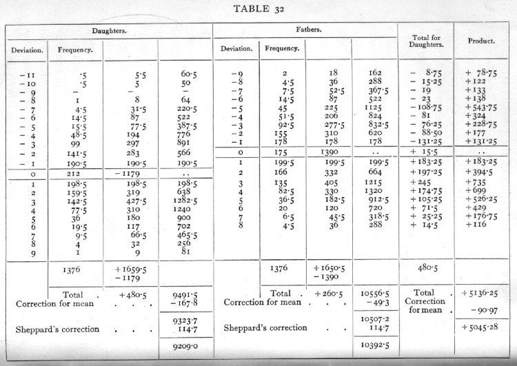
The 9th column shows the total deviations of the daughter's height for each of the 18 columns in which the table is divided. When the numbers are small, these may usually be written down by inspection of the table. In the present case, where the numbers are large, and the entries are complicated by quartering, more care is required. The total of column 9 checks with that of the 3rd column. In order that it shall do so, the central entry +15.5, Which does not contribute to the products, has to be included. Each entry in the 9th column is multiplied by the paternal deviation to give the 10th column. In the present case all the entries in column 10 are positive; frequently both positive and negative entries occur, and it is then convenient to form a separate column for each. A useful check is afforded by repeating the work of the last two columns, interchanging the variates; we should then find the total deviation of the fathers for each array of daughters, and multiply by the daughters deviation. The uncorrected totals, 5136.25, should then agree. This check is especially useful with small tables, in which the work of the last two columns, carried out rapidly, is liable to error.
The value of the correlation coefficient, using Sheppard's correction, is found by dividing 5045.28 [p. 150] by the geometric mean of 9209.0 and 10,392.5; its value is +.5157· If Sheppard's correction had not been used, we should have obtained +.5097. The difference is in this case not large compared to the errors of random sampling, and the full effects on the distribution in random samples of using Sheppard's correction have never been fully examined, but there can be little doubt that Sheppard's correction should be used, and that its use gives generally an improved estimate of the correlation. On the other hand, the distribution in random samples of the uncorrected value is simpler and better understood, so that the uncorrected value should be used in tests of significance, in which the effect of correction need not, of course, be overlooked. For simplicity coarse grouping should be avoided where such tests are intended. The fact that with small samples the correlation obtained by the use of Sheppard's correction may exceed unity, illustrates the disturbance introduced into the random sampling distribution.
32. Partial Correlations
A great extension of the utility of the idea of correlation lies in its application to groups of more than two variates. In such cases, where the correlation between each pair of three variates is known, it is possible to eliminate any one of them, and so find what the correlation of the other two would be in a population selected so that the third variate was constant.
Ex. 26. Elimination of age in organic correlations [p. 151] with growing children. -- For example, it was found (Mumford and Young's data) in a group of boys of different ages, that the correlation of standing height with chest girth was +.836. One might expect that part of this association was due to general growth with age. It would be more desirable for many purposes to know the correlation between the variates for boys of a given age; but in fact only a few of the boys will be exactly of the same age, and even if we make age groups as broad as a year, we shall have in each group much fewer than the total number measured. In order to utilise the whole material, we only need to know the correlations of standing height with age, and of chest girth with age. These are given as .714 and .708.·
The fundamental formula in calculating partial correlation coefficients may be written

Here the three variates are numbered 1, 2, and 3, and we wish to find the correlation between 1 and 2, when 3 is eliminated; this is called the "partial" correlation between 1 and 2, and is designated by r12. 3, to show that variate 3 has been eliminated. The symbols r12, r13, r23, indicate the correlations found directly between each pair of variates; these correlations being distinguished as "total" correlations.
Inserting the numerical values in the above formula we find r12. 3 =·.668, showing that when age is eliminated the correlation, though still considerable, [p. 152] has been markedly reduced. The mean value given by the above-mentioned authors for the correlations found by grouping the boys by years, is .653, not a greatly different value. In a similar manner, two or more variates may be eliminated in succession; thus with four variates, we may first eliminate variate 4, by thrice applying the above formula to find r12. 4, r13. 4, and r23. 4. Then applying the same formula again, to these three new values, we have

The labour increases rapidly with the number of variates to be eliminated. To eliminate s variates, the number of operations involved, each one application of the above formula is 1/6 s(s+1)(s+2); for values of s from 1 to 6 this gives 1, 4, 10, 20, 35, 56 operations. Much of this labour may be saved by using tables of [sqrt]1-r2 such as that published by J. R. Miner.[1]
The meaning of the correlation coefficient should be borne clearly in mind. The original aim to measure the "strength of heredity" by this method was based clearly on the supposition that the whole class of factors which tend to make relatives alike, in contrast to the unlikeness of unrelated persons, may be grouped together as heredity. That this is so for all practical purposes is, I believe, admitted, but the correlation does not tell us that this is so; it merely [p. 153] tells us the degree of resemblance in the actual population studied, between father and daughter. It tells us to what extent the height of the father is relevant information respecting the height of the daughter, or, otherwise interpreted, it tells us the relative importance of the factors which act alike upon the heights of father and daughter, compared to the totality of factors at work. If we know that B is caused by A, together with other factors independent of A, and that B has no influence on A, then the correlation between A and B does tell us how important, in relation to the other causes at work, is the influence of A. If we have not such knowledge, the correlation does not tell us whether A causes B, or B causes A, or whether both influences are at work, together with the effects of common causes.
This is true equally of partial correlations. If we know that a phenomenon A is not itself influential in determining certain other phenomena B, C, D, ..., but on the contrary is probably directly influenced by them, then the calculation of the partial correlations A with B, C, D, ... in each case eliminating the remaining values, will form a most valuable analysis of the causation of A. If on the contrary we choose a group of social phenomena with no antecedent knowledge of the causation or absence of causation among them, then the calculation of correlation coefficients, total or partial, will not advance us a step towards evaluating the importance of the causes at work.
The correlation between A and B measures, on a [p. 154] conventional scale, the importance of the factors which (on a balance of like and unlike action) act alike in both A and B, as against the remaining factors which affect A and B independently. If we eliminate a third variate C, we are removing from the comparison all those factors which become inoperative when C is fixed. If these are only those which affect A and B independently, then the correlation between A and B, whether positive or negative, will be numerically increased. We shall have eliminated irrelevant disturbing factors, and obtained, as it were, a better controlled experiment. We may also require to eliminate C if these factors act alike, or oppositely on the two variates correlated; in such a case the variability of C actually masks the effect we wish to investigate. Thirdly, C may be one of the chain of events by the mediation of which A affects B, or vice versa. The extent to which C is the channel through which the influence passes may be estimated by eliminating C; as one may demonstrate the small effect of latent factors in human heredity by finding the correlation of grandparent and grandchild, eliminating the intermediate parent. In no case, however, can we judge whether or not it is profitable to eliminate a certain variate unless we know, or are willing to assume, a qualitative scheme of causation. For the purely descriptive purpose of specifying a population in respect of a number of variates, either partial or total correlations are effective, and correlations of either type may be of interest.
As an illustration we may consider in what sense [p. 155] the coefficient of correlation does measure the "strength of heredity," assuming that heredity only is concerned in causing the resemblance between relatives; that is, that any environmental effects are distributed at haphazard. In the first place, we may note that if such environmental effects are increased in magnitude, the correlations would be reduced ; thus the same population, genetically speaking, would show higher correlations if reared under relatively uniform nutritional conditions, than they would if the nutritional conditions had been very diverse; although the genetical processes in the two cases were identical. Secondly, if environmental effects were at all influential (as in the population studied seems not to be indeed the case), we should obtain higher correlations from a mixed population of genetically very diverse strains, than we should from a more uniform population. Thirdly, although the influence of father on daughter is in a certain sense direct, in that the father contributes to the germinal composition of his daughter, we must not assume that this fact is necessarily the cause of the whole of the correlation; for it has been shown that husband and wife also show considerable resemblance in stature, and consequently taller fathers tend to have taller daughters partly because they choose, or are chosen by, taller wives. For this reason, for example, we should expect to find a noticeable positive correlation between step-fathers and step-daughters; also that, when the stature of the wife is eliminated, the partial correlation between father and daughter will be found to be lower than the total correlation. [p. 156] These considerations serve to some extent to define the sense in which the somewhat vague phrase, "strength of heredity," must be interpreted, in speaking of the correlation coefficient. It will readily be understood that, in less well understood cases, analogous considerations may be of some importance, and should if possible be critically considered.
33. Accuracy of the Correlation Coefficient
With large samples, and moderate or small correlations, the correlation obtained from a sample of n pairs of values is distributed normally about the true value r, with variance,

it is therefore usual to attach to an observed value r, a standard error (1-r2)/[srqt]n-1, or (1-r2)/[sqrt]n. This procedure is only valid under the restrictions stated above; with small samples the value of r is often very different from the true value, r, and the factor 1-r2, correspondingly in error; in addition the distribution of r is far from normal, so that tests of significance based on the above formula are often very deceptive. Since it is with small samples, less than 100, that the practical research worker ordinarily wishes to use the correlation coefficient, we shall give an account of more accurate methods of handling the results.
In all cases the procedure is alike for total and for partial correlations. Exact account may be taken of the differences in the distributions in the two cases, [p. 157] by deducting unity from the sample number for each variate eliminated; thus a partial correlation found by eliminating three variates, and based on data giving 13 values for each variate, is distributed exactly as is a total correlation based on 10 pairs of values.
34. The Significance of an Observed Correlation
In testing the significance of an observed correlation we require to calculate the probability that such a correlation should arise, by random sampling, from an uncorrelated population. If the probability is low we regard the correlation as significant. The table of t given at the end of the preceding chapter (p. 137) may be utilised to make an exact test. If n' be the number of pairs of observations on which the correlation is based, and r the correlation obtained, without using Sheppard's correction, then we take

and it may be demonstrated that the distribution of t so calculated, will agree with that given in the table.
It should be observed that this test, as is obviously necessary, is identical with that given in the last chapter for testing whether or not the linear regression coefficient differs significantly from zero.
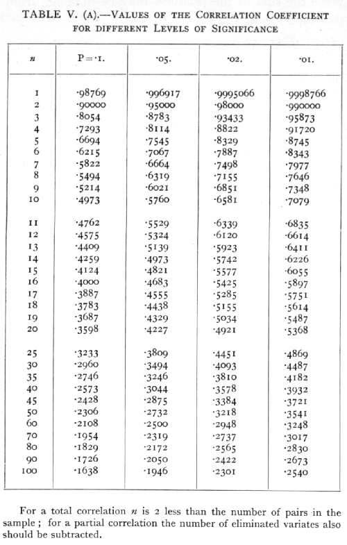
TABLE V.A (p. 174) allows this test to be applied directly from the value of r, for samples up to 100 pairs of observations. Taking the four definite levels [p. 158] of significance, represented by P =·.10, .05, .02, and .01, the table shows for each value of n, from 1 to 20, and thence by larger intervals to 100, the corresponding values of r.
Ex. 27. Significance of a correlation coefficient between autumn rainfall and wheat crop. -- For the twenty years, 1885-1904, the mean wheat yield of Eastern England was found to be correlated with the autumn rainfall; the correlation found was -.629. Is this value significant? We obtain in succession
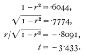
For n=18, this shows that P is less than .01, and the correlation is definitely significant. The same conclusion may be read off at once from Table V.A entered with n=18.
If we had applied the standard error,
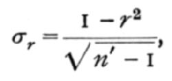
we should have

a much greater value than the true one, very much exaggerating the significance. In addition, assuming that r was normally distributed (n = [infinity]), the significance of the result would between further exaggerated. This illustration will suffice to show how deceptive, in small samples, is the use of the standard error of the [p. 159] correlation coefficient, on the assumption that it will be normally distributed. Without this assumption the standard error is without utility. The misleading character of the formula is increased if n' is substituted for n'-1, as is often done. Judging from the normal deviate 4.536, we should suppose that the correlation obtained would be exceeded in random samples from uncorrelated material only 6 times in a million trials. Actually it would be exceeded about 3000 times in a million trials, or with 500 times the frequency supposed.
It is necessary to warn the student emphatically against the misleading character of the standard error of the correlation coefficient deduced from a small sample, because the principal utility of the correlation coefficient lies in its application to subjects of which little is known, and upon which the data are relatively scanty. With extensive material appropriate for biometrical investigations there is little danger of false conclusions being drawn, whereas with the comparatively few cases to which the experimenter must often look for guidance, the uncritical application of methods standardised in biometry, must be so frequently misleading as to endanger the credit of this most valuable weapon of research. It is not true, as the above example shows, that valid conclusions cannot be drawn from small samples; if accurate methods are used in calculating the probability, we thereby make full allowance for the size of the sample, and should be influenced in our judgment only by the value of the-probability indicated. The great increase of certainty which accrues from increasing data is [p. 160] reflected in the value of P, if accurate methods are used.
Ex. 28. Significance of a partial correlation coefficient. -- In a group of 32 poor law relief unions, Yule found that the percentage change from 1881 to 1891 in the percentage of the population in receipt of relief was correlated with the corresponding change in the ratio of the numbers given outdoor relief to the numbers relieved in the workhouse, when two other variates had been eliminated, namely, the corresponding changes in the percentage of the population over 65, and in the population itself.
The correlation found by Yule after eliminating the two variates was +.457; such a correlation is termed a partial correlation of the second order. Test its significance.
It has been demonstrated that the distribution in random samples of partial correlation coefficients may be derived from that of total correlation coefficients merely by deducting from the number of the sample, the number of variates eliminated. Deducting 2 from the 32 unions used, we have 30 as the effective number of the sample; hence
n=28
Calculating t from r as before, we find
t=2.719,
whence it appears from the table that P lies between .02 and .01. The correlation is therefore significant. This, of course, as in other cases, is on the assumption [p. 161] that the variates correlated (but not necessarily those eliminated) are normally distributed; economic variates seldom themselves give normal distributions, but the fact that we are here dealing with rates of change makes the assumption of normal distribution much more plausible. The values given in Table V.(A) for n=25, and n=30, give a sufficient indication of the level of significance attained by this observation.
35. Transformed Correlations
In addition to testing the significance of a correlation, to ascertain if there is any substantial evidence of association at all, it is also frequently required to perform one or more of the following operations, for each of which the standard error would be used in the case of a normally distributed quantity. With correlations derived from large samples the standard error may, therefore, be so used, except when the correlation approaches [plus or minus]1; but with small samples such as frequently occur in practice, special methods must be applied to obtain reliable results.
(i.) To test if an observed correlation differs significantly from a given theoretical value.
(ii.) To test if two observed correlations are significantly different.
(iii.) If a number of independent estimates of a correlation are available, to combine them into an improved estimate.
(iv.) To perform tests (i.) and (ii.) with such average values. [p. 162]
Problems of these kinds may be solved by a method analogous to that by which we have solved the problem of testing the significance of an observed correlation. In that case we were able from the given value r to calculate a quantity t which is distributed in a known manner, for which tables were available. The transformation led exactly to a distribution which had already been studied. The transformation which we shall now employ leads approximately to the normal distribution in which all the above tests may be carried out without difficulty. Let
z = ½{loge(1+r) - loge(1-r)}
then as r changes from 0 to 1, z will pass from 0 to [infinity]. For small values of r, z is nearly equal to r, but as r approaches unity, z increases without limit. For negative values of r, z is negative. The advantage of this transformation lies in the distribution of the two quantities in random samples. The standard deviation of r depends on the true value of the correlation, r; as is seen from the formula
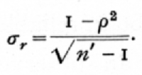
Since r is unknown, we have to substitute for it the observed value r, and this value will not, in small samples, be a very accurate estimate of r. The standard error of z is simpler in form,

and is practically independent of the value of the [p. 163] correlation in the population from which the sample is drawn.
In the second place the distribution of r is skew in small samples, and even for large samples it remains very skew for high correlations. The distribution of z is not strictly normal, but it tends to normality rapidly as the sample is increased, whatever may be the value of the correlation. We shall give examples to test the effect of the departure of the z distribution from normality.
Finally the distribution of r changes its form rapidly as r is changed ; consequently no attempt can be made, with reasonable hope of success, to allow for the skewness of the distribution. On the contrary, the distribution of z is nearly constant in form, and the accuracy of tests may be improved by small corrections for skewness; such corrections are, however, in any case somewhat laborious, and we shall not deal with them. The simple assumption that z is normally distributed will in all ordinary cases be sufficiently accurate.
These three advantages of the transformation from r to z may be seen by comparing Figs. 7 and 8. In Fig. 7 are shown the actual distributions of r, for 8 pairs of observations, from populations having correlations 0 and 0.8; Fig. 8 shows the corresponding distribution curves for z. The two curves in Fig. 7 are widely different in their modal heights; both are distinctly non-normal curves; in form also they are strongly contrasted, the one being symmetrical, the other highly unsymmetrical. On the contrary, in [p. 164] Fig. 8 the two curves do not differ greatly in height; although not exactly normal in form, they come so close to it, even for a small sample of 8 pairs of observations, [p. 165] that the eye cannot detect the difference; and this approximate normality holds up to the extreme limits r=[plus or minus]1. One additional feature is brought out by Fig. 8 ; in the distribution for r=0.8, although the curve itself is as symmetrical as the eye can judge of, yet the ordinate of zero error is not centrally placed. The figure, in fact, reveals the small bias which is introduced into the estimate of the correlation coefficient as ordinarily calculated; we shall treat further of this bias in the next section, and in the following chapter shall deal with a similar bias introduced in the calculation of intraclass correlations.

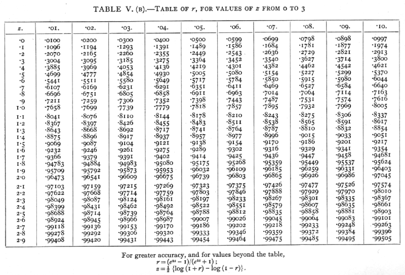
To facilitate the transformation we give in Table V.(B) (p. 175) the values of r corresponding to values of z, proceeding by intervals of ,01, from 0 to 3. In the earlier part of this table it will be seen that the values of r and z do not differ greatly; but with higher correlations small changes in r correspond to relatively large changes in z. In fact, measured on the z-scale, a correlation of .99 differs from a correlation .95 by more than a correlation .6 exceeds zero. The values of z give a truer picture of the relative importance of correlations of different sizes, than do the values of r.
To find the value of z corresponding to a given value of r, say .6, the entries in the table lying on either side of .6, are first found, whence we see at once that z lies between .69 and .70; the interval between these entries is then divided proportionately to find the fraction to be added to .69. In this case we have 20/64, or .31, so that z=.6931. Similarly, in finding [p. 166] the value of r corresponding to any value of z, say .9218, we see at once that it lies between .7259 and .7306; the difference is 47, and 18 per cent of this gives 8 to be added to the former value, giving us finally r=.7267. The same table may thus be used to transform r into z, and to reverse the process.
Ex. 29. Test of the approximate normality of the distribution of z. -- In order to illustrate the kind of accuracy obtainable by the use of z, let us take the case that has already been treated by an exact method in Ex. 26. A correlation of -.629 has been obtained from 20 pairs of observations ; test its significance.
For r=-.629 we have, using either a table of natural logarithms, or the special table for z, z=.7398. To divide this by its standard error is equivalent to multiplying it by [sqrt]17.· This gives -3.050, which we interpret as a normal deviate. From the table of normal deviates it appears that this value will be exceeded about 23 times in 10,000 trials. The true frequency, as we have seen, is about 30 times in 10,000 trials. The error tends slightly to exaggerate the significance of the result.
Ex. 30.· Further test of the normality of the distribution of z. -- A partial correlation +.457 was obtained from a sample of 32, after eliminating two variates. Does this differ significantly from zero? Here z =.4935; deducting the two eliminated variates the effective size of the sample is 30, and the standard error of z is 1/[sqrt]27; multiplying z by [sqrt]27, we have as a. normal variate 2.564. Table IV. shows, as before, that P is just over ·.01. There is a slight exaggeration [p. 167] of significance, but it is even slighter than in the previous example.
The above examples show that the z transformation will give a variate which, for most practical purposes, may be taken to be normally distributed. In the case of simple tests of significance the use of the table of t is to be preferred ; in the following examples this method is not available, and the only method available which is both tolerably accurate and sufficiently rapid for practical use lies in the use of z.
Ex. 31· Significance of deviation from expectation of an observed correlation coefficient. -- In a sample of 25 pairs of parent and child the correlation was found to be .60. Is this value consistent with the view that the true correlation in that character was .46?
The first step is to find the difference of the corresponding values of z. This is shown below:
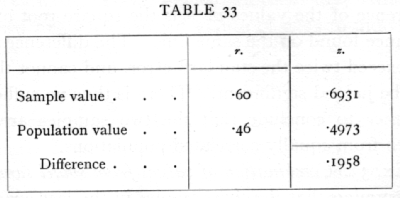
To obtain the normal deviate we multiply by [sqrt]22, and obtain .918. The deviation is less than the standard deviation, and the value obtained is therefore quite in accordance with the hypothesis. [p. 168]
Ex. 32. Significance of difference between two observed correlations. -- Of two samples the first, of 20 pairs, gives a correlation .6, the second, of 25 pairs, gives a correlation .8: are these values significantly different?
In this case we require not only the difference of the values of z, but the standard error of the difference. The variance of the difference is the sum of the reciprocals of 17 and 22; the work is shown below:

The standard error which is appended to the difference of the values of z is the square root of the variance found on the same line. The difference does not exceed twice the standard error, and cannot therefore be judged significant. There is thus no sufficient evidence to conclude that the two samples are not drawn from equally correlated populations.
Ex. 33· Combination of values from small samples. -- Assuming that the two samples in the last example were drawn from equally correlated populations, estimate the value of the correlation.
The two values of z must be given weight inversely proportional to their variance. We therefore [p. 169] multiply the first by 17, the second by 22 and add, dividing the total by 39. This gives an estimated value of z for the population, and the corresponding value of r may be found from the table.
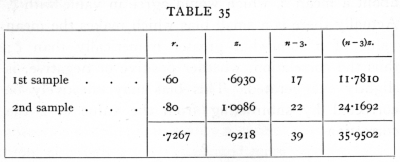
The weighted average value of z is .9218, to which corresponds the value r=.7267; the value of z so obtained may be regarded as subject to normally distributed errors of random sampling with variance equal to 1/39· The accuracy is therefore equivalent to that of a single value obtained from 42 pairs of observations. Tests of significance may thus be applied to such averaged values of z, as to individual values.
36. Systematic Errors
In connexion with the averaging of correlations obtained from small samples it is worth while to consider the effects of two classes of systematic errors, which, although of little or no importance when single values only are available, become of increasing importance as larger numbers of samples are averaged.
The value of z obtained from any sample is an estimate of a true value, r, belonging to the sampled [p. 170] population, just as the value of r obtained from a sample is an estimate of a population value, r. If the method of obtaining the correlation were free from bias, the values of z would be normally distributed about a mean z[bar], which would agree in value with z. Actually there is a small bias which makes the mean value of z somewhat greater numerically than z; thus the correlation, whether positive or negative, is slightly exaggerated. This bias may effectively be corrected by subtracting from the value of z the correction

For single samples this correction is unimportant, being small compared to the standard error of z. For example, if n'=10, the standard error of z is .378, while the correction is r/l8 and cannot exceed .056. If, however, z[bar] were the mean of 1000 such values of z, derived from samples of 10, the standard error of z[bar] is only .012, and the correction, which is unaltered by taking the mean, may become of great importance.
The second type of systematic error is that introduced by neglecting Sheppard's correction. In calculating the value of z, we must always take the value of r found without using Sheppard's correction, since the latter complicates the distribution.
But the omission of Sheppard's correction introduces a systematic error, in the opposite direction to that mentioned above; and which, though normally very small, appears in large as well as in small samples. In case of averaging the correlations from a number of [p. 171] coarsely grouped small samples, the average z should be obtained from values of r found without Sheppard's correction, and to the result a correction, representing the average effect of Sheppard's correction, may be applied.
37. Correlation between Series
The extremely useful case in which it is required to find the correlation between two series of quantities, such as annual figures, arranged in order at equal intervals of time, is in reality a case of partial correlation, although it may be treated more directly by the method of fitting curved regression lines given in the last chapter (p. 128).
If, for example, we had a record of the number of deaths from a certain disease for successive years, and wished to study if this mortality were associated with meteorological conditions, or the incidence of some other disease, or the mortality of some other age group, the outstanding difficulty in the direct application of the correlation coefficient is that the number of deaths considered probably exhibits a progressive change during the period available. Such changes may be due to changes in the population among which the deaths occur, whether it be the total population of a district, or that of a particular age group, or to changes in the sanitary conditions in which the population lives, or in the skill and availability of medical assistance, or to changes in the racial or genetic composition of the population. In any case it is usually found that the changes are still apparent [p. 172] when the number of deaths is converted into a death-rate on the existing population in each year, by which means one of the direct effects of changing population is eliminated.
If the progressive change could be represented effectively by a straight line it would be sufficient to consider the time as a third variate, and to eliminate it by calculating the corresponding partial correlation coefficient. Usually, however, the change is not so simple, and would need an expression involving the square and higher powers of the time adequately to represent it. The partial correlation required is one found by eliminating not only t, but t2, t3, t4, ..., regarding these as separate variates; for if we have eliminated all of these up to (say) the fourth degree, we have incidentally eliminated from the correlation any function of the time of the fourth degree, including that by which the progressive change is best represented.
This partial correlation may be calculated directly from the coefficients of the regression function obtained as in the last chapter (p. 128). If y and y' are the two quantities to be correlated, we obtain for y the coefficients A, B, C,..., and for y' the corresponding coefficients A', B', C', .. .; the sum of the squares of the deviations of the variates from the curved regression lines are obtained as before, from the equations
 [p. 173]
while the sum of the products may be obtained from the similar equation

the required partial correlation being, then,

In this process the number of variates eliminated is equal to the degree of t to which the fitting has been carried; it will be understood that both variates must be fitted to the same degree, even if one of them is capable of adequate representation by a curve of lower degree than is the other. [p. 174]
 [p. 175]
Footnotes
[1] Tables of [sqrt]1-r2 for Use in Partial Correlation, and in Trigonometry. Johns Hopkins Press, 1922.