FourierSeries.html

FourierSeries.html FourierSeries.mws

Fourier series

In the worksheet HeatEqn.mws we have seen how a partial differential equation (the heat equation) in one space and one time dimension admitted solutions in product form (separation of variables technique), and how the solution was approximated by expanding the spatial part in a Fourier sine series. In this worksheet we generalize the idea of representing functions defined on a finite interval (part of the real axis) by means of an expansion in basis functions. The concepts can then be extended to basis functions defined as the eigenfunctions of some Sturm-Liouville operator.

We begin by defining our basic interval on which the function is to be defined. This would normally be the interval on which solutions to a differential equation are seeked, i.e., usually the unknown function (solution to the ODE) has specified values at the edges of the interval. The choice of a and b below is arbitrary, and depends on the problem posed. In quantum mechanics we could be asking for particles to be located in a box bounded by these edges.

> restart; a:=-2; b:=3;

We define an inner product for real-valued functions (without weight function) assuming that the independent variable is called x :

> IP:=(f,g)->int(expand(f*g),x=a..b);

This inner (dot) product will be used to calculate the norm of functions, and the projection of functions onto basis functions. The expand function has been included to help Maple calculate integrals by breaking them into many simpler pieces.

The basis will be defined as the eigenfunctions of the following simple differential operator:

> DO:=f->-diff(f,x$2);

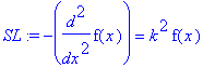
In order to determine the eigenfunctions and eigenvalues of this differential operator on the interval [a,b] we have to specify some boundary conditions (BC). We anticipate (based on elementary Calculus) that sin(k*x) and cos(k*x) are candidates for the eigenfunctions, and that k^2 will appear as an eigenvalue. The boundary conditions will impose which values of k are permitted.

In the example carried out in HeatEqn.mws we encountered two types of BCs: we can fix the value of the basis function, or we can fix its derivative.

The eigenvalue problem

DO(f) = lambda*f , lambda=k^2

is homogeneous, which means that if f(x) is a solution, then any multiple of it will be a solution as well.

If we do not impose boundary conditions, then the value of k will be unrestricted, and the interval [a,b] becomes somehow irrelevant. This means that the functions are defined on the entire real axis (something which becomes important in quantum mechanics when discussing plane-wave free-particle solutions).

Let us start with the simple case of imposing that the basis functions vanish at both a and b . These BCs are called homogeneous.

> BC1:=f(a)=0;

> SL:=DO(f(x))=k^2*f(x);

How do we find the basis functions that satisfy this equation? We can't use the second boundary condition, because that would force the boring trivial solution f(x)=0 . We have to use the choice of eigenvalue lambda to find non-trivial solutions.

> sol:=dsolve({SL,BC1},f(x));

The choice of integration constant _C1 is arbitrary and defines the normalization of the solution. We impose now the second boundary condition:

> fB:=subs(_C1=1,rhs(sol));

> BC2:=subs(x=b,fB)=0;

This is a nonlinear transcendental equation which admits infinitely many roots. To find the roots we have to employ a numerical solver. First, let us graph the expression whose roots we are seeking.

> plot(lhs(BC2),k=-5..5,view=[-5..5,-4..4],discont=true);

Clearly, we need to consider k >= 0 only. The functions are labelled by eigenvalue k^2 , which cannot distinguish positive from negative values.

The poles that appear in-between the roots can make life difficult for a systematic root search, but at least it is clear where they occur, as they are associated with tan(2*k) , i.e., they occur for 2*k = m*Pi , where m=1,2,...

The root k = 0 does not lead to an interesting solution (due to the homogeneous BCs imposed we don't have a constant term).

The expression is periodic in k with period 2*Pi .

> k1:=fsolve(BC2,k=0.0001..Pi/4-0.0001);

> k2:=fsolve(BC2,k=Pi/4+0.0001..Pi/2);

> k3:=fsolve(BC2,k=Pi/2..3*Pi/4-0.0001);

> k4:=fsolve(BC2,k=2..3);

> k5:=fsolve(BC2,k=3*Pi/4..5*Pi/4);

> k6:=fsolve(BC2,k=Pi+0.0001..5*Pi/4);

> evalf(k6-Pi),k1;

Maple's solve command finds analytic expressions for the roots:

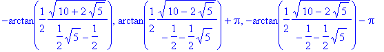
> sol:=solve(BC2,k);

> simplify(sol[3]);

> evalf(sol);

We will be content with using the first five basis states, but the periodicity allows one to construct all other eigenvalues easily from the five numbers k1..k5 .

Let us graph the basis states:

> plot([seq(subs(k=k||j,fB),j=1..5)],x=a..b,color=[red,blue,green,black,brown]);

We recognize that there are sine-type and cosine-type solutions present by looking at the behaviour with respect to x=0 .

> Bf:=i->subs(k=k||i,fB);

> IP(Bf(1),Bf(1));

> IP(Bf(2),Bf(2));

The functions are not normalized yet.

> IP(Bf(1),Bf(2));

> IP(Bf(1),Bf(3));

> IP(Bf(2),Bf(3));

They are orthogonal within numerical accuracy (numerics come into play due to the approximate nature of the eigenvalues).

We can generate a list of normalized eigenfunctions:

> Bfn:=[seq(Bf(i)/sqrt(IP(Bf(i),Bf(i))),i=1..5)];

> plot(Bfn,x=a..b,color=[red,blue,green,black,brown]);

Now let us expand some known functions in this basis. We begin with a function that satisfies the boundary conditions obeyed by the basis.

> f1:=(x-a)^3*(x-b)^2;

> plot(f1,x=a..b);

The expansion coefficients are obtained by projection:

> c_n:=[seq(IP(f1,Bfn[j]),j=1..5)];

> f1_ap:=add(c_n[n]*Bfn[n],n=1..5);

> plot([f1,f1_ap],x=a..b,color=[red,blue]);

Five basis functions are sufficient to reach almost 1%-level accuracy!

Exercise 1:

Change the power for the (x-a) and (x-b) factors and repeat the calculation with five basis states. What do you observe?

Exercise 2:

Increase the order of the expansion by finding the next five eigenvalues (you can use the periodicity), and eigenfunctions. Does the convergence behaviour become evident?

This was an example of applying linear algebra techniques to a function space. We used an eigenvalue problem to define a set of eigenvectors (basis functions), and then we expanded some arbitrary vector (function) in this basis. The economy is obvious: we can have approximate knowledge of a function by knowing a set of numbers (the expansion coefficients). Often one can adapt a basis to a problem at hand, and, thus, limit the number of expansion coefficients required for a reasonably accurate representation.

We demonstrate now what happens when we look outside the interval [a,b]:

> plot([f1,f1_ap],x=-10..10,color=[red,blue],view=[-10..10,-200..200],numpoints=500);

We observe that the answer obtained from the Fourier series is periodic, i.e., it repeats itself outside the interval [a,b].

Exercise 3:

Change the interval [a,b] to cover a wider range (e.g., [-3,4]), repeat the calculation for the Fourier series, and make your observation. Investigate the convergence behaviour.

For functions that do not vanish on the edge of the interval some interesting pheonomena can be observed. The textbooks on the subject develop the calculation of Fourier coefficients for simple periodic functions (square wave train, sawtooth function, etc.), for which a formula for the expansion coefficients can be derived. This permits to study convergence behaviour in a straightforward way.

Let us define the next wavenumbers for the Fourier basis. We found k5 to be related to k1.

> plot(lhs(BC2),k=0..9,view=[0..9,-4..4],discont=true);

> k6;

> k7:=fsolve(BC2,k=4.1..4.8);

> k8:=fsolve(BC2,k=4.8..5.5);

> k9:=fsolve(BC2,k=5.5..6);

> k10:=fsolve(BC2,k=6..6.5);

> k11:=k1+evalf(2*Pi);

> k12:=k2+evalf(2*Pi);

> k13:=k3+evalf(2*Pi);

> k14:=k4+evalf(2*Pi);

> k15:=k5+evalf(2*Pi);

> k16:=k6+evalf(2*Pi);

> plot([seq([n,k||n],n=1..16)],style=point);

> k1,k2-k1,k3-k2,k4-k3,k5-k4,k6-k5;

We can actually infer the behaviour of the eigenvalues as a function of order:

> evalf(2*Pi/10);

Now we are able to carry out a limited convergence study. Let us pick an arbitrary function, and expand it over [a,b].

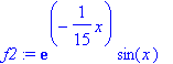
> f2:=exp(-x/15)*sin(x);

> Bfn:=[seq(Bf(i)/sqrt(IP(Bf(i),Bf(i))),i=1..15)]:

> c_n:=[seq(IP(f2,Bfn[j]),j=1..15)];

> f2_ap5:=add(c_n[n]*Bfn[n],n=1..5):

> f2_ap10:=add(c_n[n]*Bfn[n],n=1..10):

> f2_ap15:=add(c_n[n]*Bfn[n],n=1..15):

> plot([f2_ap5,f2_ap10,f2_ap15,f2],x=a..b,color=[red,blue,green,black]);

What happens at the left-hand side is known as the Gibbs phenomenon. Given that all basis functions vanish at x=a and at x=b , the approximate Fourier series representation cannot be accurate there. The Fourier expansion tries to approximate a step function behaviour: at the endpoints the function is assumed to rise immediately to the non-zero value with infinite slope. Fourier expansions with a large number of terms are able to produce a large slope, but the price is paid by the wiggling around the true function even some distance away from the boundary.

Exercise 4:

Use the analytic expression found for the values of k||n to push the expansion to high order (e.g., n_max=50 ) and observe the Gibbs phenomenon.

Solution of a differential equation

So far we have not calculated anything particularly useful given that the functions to be represented could be easily expressed as elementary expressions. We will show now that the Fourier series expansion allows to convert differential equation problems into linear algebra assignments.

Let us define an inhomogeneous linear second-order differential equation with boundary conditions specified at the ends of the interval [a,b].

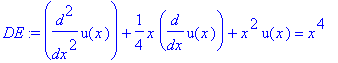
> DE:=diff(u(x),x$2)+1/4*x*diff(u(x),x)+x^2*u(x)=x^4;

> BCd:=u(a)=0,u(b)=0;

> solDE:=dsolve({DE,BCd},u(x));

Maple can't solve this one. We can generate a numerical solution to this boundary value problem using the dsolve[numeric] integrator.

> solDE:=dsolve({DE,BCd},u(x),numeric,output=listprocedure):

> U:=subs(solDE,u(x)):

> plot(U(x),x=a..b);

Now we produce a basis-expansion solution. We generate a matrix from the left-hand side of the equation by acting with the differential operator on basis function Bfn[j], while multiplying with Bfn[i] and integrating.

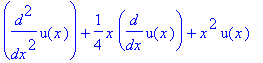
> lhs(DE);

> Nb:=9;

> with(LinearAlgebra):

> A:=Matrix(Nb,Nb):

> for i from 1 to Nb do: for j from 1 to Nb do: A[i,j]:=IP(Bfn[i],subs(u(x)=Bfn[j],lhs(DE))): od: od:

> evalm(A);

> Ai:=MatrixInverse(A);

Now we form a right-hand-side vector using a projection of the rhs of the ODE onto the basis states:

> bvec:=Vector(Nb):

> for i from 1 to Nb do: bvec[i]:=IP(rhs(DE),Bfn[i]): od:

> evalm(bvec);

> cvec:= Ai . bvec;

> solAP:=add(cvec[i]*Bfn[i],i=1..Nb):

> plot([solAP,U(x)],x=a..b,color=[red,blue]);

Exercise 5:

Pick a linear differential equation of your choice with appropriate boundary conditions and compare numerical solutions as provided by Maple with the Fourier-series solution. Observe the efficiency of the Fourier method: the solution is specified using a small number of real coefficients.

Solution of a differential equation - eigenvalue problem

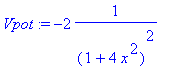
Here we apply the Fourier-series expansion technique to a Schroedinger equation. This will result in a matrix eigenvalue problem. We will continue to use our asymmetric interval [a,b], but apply it to a situation where a symmetric interval would be more appropriate. We cosnsider the bound states in a potential that has an inverted bell shape:

> Vpot:=-2/(1+(2*x)^2)^2;

> plot(Vpot,x=a..b);

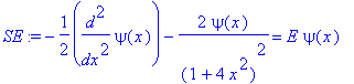
We will ask the following question: Given that the kinetic energy can be represented as

Tkin = - 1/2 diff(psi(x),x$2)

what are the allowed energy eigenvalues for Tkin+Vpot ? [for physicists: we have chosen units in which Planck's constant h=2*Pi , and the mass of the particle equals unity, and a third constant was chosen so that the strength of the potential energy is dimensonless]. The kinetic energy operator represents p^2/(2*m) using the association (prescription) that p = - I*h/(2*Pi)*d/dx

> SE:=-1/2*diff(psi(x),x$2)+Vpot*psi(x) = E*psi(x);

We are looking for bound solutions, i.e., E < 0 . The ODE problem is homogeneous (eigenvalue problems always are). This problem cannot be solved easily by dsolve[numeric], because the energy eigenvalue is unknown a priori.

We generate a matrix representation as before:

> Nb:=5;

> A:=Matrix(Nb,Nb):

> for i from 1 to Nb do: for j from 1 to Nb do: A[i,j]:=IP(Bfn[i],subs(psi(x)=Bfn[j],lhs(SE))): print(i,j,A[i,j]); od: od:

> evalm(A);

What do we notice?

1) the imaginary part in the matrix elements looks like spurious noise

2) the matrix is almost symmetric [the small deviations are a result of using non-symmetric boundary conditions in the basis]

Before we proceed with finding the eigenvalues we correct the two problems:

> A:=map(Re,A);

> A:=0.5*(A + Transpose(A));

> Eigenvalues(A);

We have found one bound state. To determine how reliable the energy estimate is we have to increase the matrix size and repeat the calculation.

E0 = -.52511 from 4-by-4 ( Nb=4 )

E0 = -.54981 from 9-by-9 ( Nb=9 )

Exercise 6:

Carry out a convergence analysis. Concentrate on the lowest-lying eigenvalue (the ground state). The higher-lying states are artificial states.

Exercise 7:

Deepen the potential well by increasing the constant that pre-multiplies the potential. Re-compute the ground state. Are there additional bound states in the potential well?

To compute the eigenfunction psi_0(x) associated with the eigenenergy E0 we have to look at the eigenvector and assemble the superposition. The syntax is somewhat cumbersome.

> EV:=Eigenvectors(A);

> n0:=1;

> EV[1][n0];

> cf:=seq(EV[2][j,n0],j=1..Nb);

> psi0:=add(Re(cf[j]*Bfn[j]),j=1..Nb):

> plot(psi0^2,x=a..b);

This is an approximation to the square of the ground-state wavefunction which (when normalized properly) carries the probability information of where to find particles in position space (if they are in the ground state). Observe carefully how the wings of the distribution are in the classically forbidden regime:

> plot([Vpot,psi0^2+EV[1][n0],EV[1][n0]],x=a..b,color=[red,blue,green]);

The baseline for the wavefunction graph intersects the potential energy at the classical turning point (all kinetic energy is converted into potential energy there).

The asymmetry is caused by the basis. For larger values of Nb the ground state is calculated to be symmetric (as it should be for a symmetric potential).

The state is actually properly normalized:

> IP(psi0,psi0);

For sufficiently deep (and wide) potentials additional bound states appear. The next bound state (first excited state) in a symmetric potential is anti-symmetric (has odd parity). The probability density (square of the wavefunction) has a node at x=0 in this case. Verify this feature on an example of your choice.

>