Torque-free gyroscope

We consider a gyroscope that has a counterweight such that the gravitational torque is balanced. Such a gyro will not precess. Now we push on the axle either gently to induce precession, or rapidly, e.g., by the blow of a hammer. This situation is considered in the text Elements of Newtonian Mechanics  by J.M. Knudsen and P.G. Hjorth (Springer-Verlag 2000, 3rd ed.) in Example 13.7. The torque-free symmetrical top is often the subject of somewhat abstract analysis demonstrating how the top's symmetry axis and the angular velocity vector precess with respect to the conserved angular momentum vector.

Our objective is to implement the equations of motion which follow from modified Euler's equations for rigid body rotation and to demonstrate the difference between pulse-shaped torques and gentle downward taps on the gyro axis. The parameters for the gyroscope are taken from a problem in the text. The gyro axle is of length l , the gyro itself is a disk of radius R , and mass M , balanced by a counterweight of equal mass at the same distance. We assume the axle to be substantially larger than the disk radius, such that the inertia about the axes perpendicular to the symmetry axis can be assumed to be 2*M*l^2 . We assume constant spin about the symmetry axis with angular velocity w0 .

>	restart; Digits:=15:

>	with(plots): with(plottools):

Warning, the name changecoords has been redefined

Warning, the name arrow has been redefined

>	M:=2.4: l:=0.3: R:=0.1:

>	w0:=200: T_rot:=6.28/w0;

An omega=200 corresponds to about 33 rps, or 1812 rpm.

>	I1:=2*M*l^2; I3:=M/2*R^2;

As derived in the notes the Euler equations are augmented by an additional term: the 'almost body frame' is defined by an angular velocity vector that excludes the spin about the symmetry axis. To account for it an omega  crossed into L_spin  term had to be added to the rate of change of angular momentum. We will specify the torque about the 1-axis later. In the true body fram the 1- and 2-axes (perpendicular to the symmetry axis labeled as the 3-axis) would be spinning around experiencing periodically modulated torques.

>	EE1:=I1*diff(w1(t),t)-(I1-I3)*w2(t)*w3(t)+I3*w0*w2(t)=N1(t);

>	EE2:=I1*diff(w2(t),t)+(I1-I3)*w1(t)*w3(t)-I3*w0*w1(t)=0;

The next equations establish the relationship of [w1, w2, w3]  to the orientation angles for the symmetry axis. The polar nutation angle is theta , and the azimuthal precession angle is phi . This relationship is established by the geometry: the body 1-axis is oriented such that rotations about it correspond to nutation in the mathematically positive sense. Depending on the nutational orientation the precession feeds partially into rotation about the 2- and 3-axes: for the horizontal orientation precession has no contribution to rotation about the symmetry axis, for the vertical orientation it adds to the spin totally. Thus: [w1, w2, w3] = [-diff(theta(t),t) , -diff(phi(t),t)*sin(theta(t) , diff(phi(t),t)*cos(theta(t)) ]   

>	OE1:=diff(theta(t),t)=-w1(t);

>	OE2:=diff(phi(t),t)=-w2(t)/sin(theta(t));

The third component of the angular velocity vector needs to be eliminated from the equations. The Euler equation of motion for the third component expresses conservation of the 3-component of angular momentum, and is not used explicitly. We solve for the two orientational degrees of freedom theta(t)  and phi(t) . Redefine the Euler equations:

>	EE1:=subs(w3(t)=diff(phi(t),t)*cos(theta(t)),EE1);

>	EE2:=subs(w3(t)=diff(phi(t),t)*cos(theta(t)),EE2);

Let us first consider the problem of the hammer blow treated not by means of a torque, but a momentum transfer. Suppose one SI unit of angular momentum is transferred into the nutational motion at time zero. Let us understand by how much the angular momentum changes in magnitude:

>	L_spin:=I3*w0;

>	L_blow:=1;

>	theta_dot:=L_blow/I1;

>	IC:=phi(0)=0,w2(0)=0,theta(0)=evalf(Pi/2),w1(0)=-theta_dot;

We selected no precessional motion at time zero. The gyro is torque-free:

>	EE10:=subs(N1(t)=0,EE1);

>	sol:=dsolve({EE10,EE2,OE1,OE2,IC},numeric,output=listprocedure):

>	Theta:=eval(theta(t),sol): Phi:=eval(phi(t),sol):

>	plot([Theta(t)-Pi/2,Phi(t)],t=0..2,color=[red,blue]);

We have the same amplitude in theta  and phi . We note that the gyroscope carries out simple periodic motion - something we might not have expected at first from the nonlinear equations.

We have chosen a massive change in angular momentum (tremendous blow compared to the spin). Considerable nutational and precessional oscillations are the result. What is remarkable is that the nutation is about the original inclination of Pi/2 , the precessional oscillation is about a displaced centre angle. The conserved angular momentum vector points downward.

An interesting question: what sets the rather long time scale for the nutational/precessional oscillations? One can derive the equations of motion for the theta and phi angles, linearize them, and show that in the limit of small-amplitude oscillations harmonic solutions exist with circular frequency Omega=I3*w0/I1 .

>	Omega:=I3*w0/I1; T_osc:=evalf(2*Pi/Omega);

Exercise 1:

Explore the motion as a function of the strength of the momentum transfer to the gyro axle (imparted angular momentum change). Find out for which range of theta  oscillations the linearized approximation is valid, i.e., the period follows the above formula. Also explore initial conditions for which the excursion amplitude in the nutation is larger than given above.

Exercise 2:

Explore the character of the motion when the gyro is not started in the horizontal orientation. This should result in motion in the nonlinear regime. How would you characterize this motion?

Can we depict the relation of the three vectors: angular momentum, angular velocity, symmetry axis as a function of time?

>

L_spin;

>	N:=300: for i from 1 to N do: t:=0.03*i: Prec:=vector([l*sin(Theta(t))*cos(Phi(t)),l*sin(Theta(t))*sin(Phi(t)),l*cos(Theta(t))]) ; ll[i] := arrow(vector([0,0,0]), Prec, .1, .4, .1): od:

>	i:='i': display3d([seq(ll[i],i=1..N)], color=red,orientation=[66,48],axes=boxed,insequence=true,scaling=constrained);

Maple programming exercise:  depict the angular velocity vector in the lab frame superimposed in the visualization of the 3-axis.

>

Now introduce a torque which can be chosen as a pulse of different length compared to the rotation period of the gyro.

>	T_rot:=6.28/w0;

Now solve with an excitation pulse:

>	N1:=t->-exp(-((t-0.15)/(1*T_rot))^4);

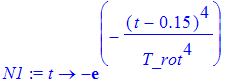
>	t:='t': plot(N1(t),t=0..1,numpoints=1000);

We change the initial conditions to imply no motion without the pulse:

>	IC:=phi(0)=0,w2(0)=0,theta(0)=evalf(Pi/2),w1(0)=0;

>	sol:=dsolve({EE1,EE2,OE1,OE2,IC},numeric,output=listprocedure):

>	Theta:=eval(theta(t),sol): Phi:=eval(phi(t),sol):

>	plot([Theta(t)-Pi/2,Phi(t)],t=0..2,color=[red,blue],numpoints=2000);

The pulse results in action very much along the lines of what we did through initial conditions above. The motion sets in at a time when the pulse gains strength.

On a technical note: if we delay the pulse to later time, dsolve[numeric]  has problems to connect the initial condition to a proper solution due to round-off.

The amplitude of oscillation is much less than before. What is the implied angular momentum change?

>	evalf(Int(N1(t),t=0..0.4));

Now repeat the procedure for a pulse that is longer-lived, and has a rise time that does not resonate.

>	N1:=t->-exp(-((t-1)/(20*T_rot))^4);

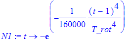
>	t:='t': plot(N1(t),t=0..2,numpoints=1000);

We change the initial conditions to imply no motion without the pulse:

>	IC:=phi(0)=0,w2(0)=0,theta(0)=evalf(Pi/2),w1(0)=0;

>	sol:=dsolve({EE1,EE2,OE1,OE2,IC},numeric,output=listprocedure):

>	Theta:=eval(theta(t),sol): Phi:=eval(phi(t),sol):

>	plot([Theta(t)-Pi/2,Phi(t)],t=0..4,color=[red,blue],numpoints=2000);

The behaviour is qualitatively different now: rather than exciting resonant oscillations in the gyroscope the rise and fall times of the pulse are so long that we have almost adiabatic motion. We can compare the situation to a mass-spring system: excitation on short time scales comparable to the natural frequency would lead to oscillations, while slow pushes would just move the mass from one equilibrium position (without force applied) to a new one (with force applied) and vice versa.

The pulsed torque is of longer duration and leads to more angular momentum change:

>	evalf(Int(N1(t),t=0..1));

In this case the angular momentum vector precessed to a new location via excursion to nutation angles below the horizontal and back. The above graph shows clearly that precession follows the nutation.

What is curious about the above discussion: the natural oscillations of the gyroscope are slow - the period is about 1.02 seconds (it is somewhat shorter than in the linearized limit). What controls whether the gyro responds by strong oscillations on this time scale or by precession with small oscillations superimposed is not resonance with this frequency, but the rise time of the pulse compared to the rotation period multiplied by some number. This number involves the ratio of moments of inertia I3/I1 . For our example this number is small (almost 1/40).

Exercise 3:

Explore the behavior of the tapped gyroscope by changing the parameters of the torque pulse.

Intellectual exercise:  compare the present approach to the direct solution of the equations of motion for theta(t)  and phi(t)  as carried out in Gyro.mws  

>

>	N:=150: for i from 1 to N do: t:=0.02*i: Prec:=vector([l*sin(Theta(t))*cos(Phi(t)),l*sin(Theta(t))*sin(Phi(t)),l*cos(Theta(t))]) ; ll[i] := arrow(vector([0,0,0]), Prec, .1, .4, .1): od:

>	i:='i': display3d([seq(ll[i],i=1..N)], color=red,orientation=[35,50],axes=boxed,insequence=true,scaling=constrained);

Mini-project:  demonstrate the time evolution of the angular momentum vector. Show how close its evolution comes to the naive treatment by the angular momentum theorem (steady precession).

>

>

>

>