Numerical solution of the Schroedinger equation for partial waves:

scattering from a spherical potential [we choose the attractive exponential potential below, but any potential can be put in]

>	restart; Digits:=14:

>

L:=0;

$L:=0$

>

k:=0.5;

$k:=.5$

>

V0:=-1;

$\mathrm{V0}:=-1$

>	V:=V0*exp(-r);

$V:=-e^{\left(-r\right)}$

>	SE:=diff(u(r),r$2)+(k^2-2*V-L*(L+1)/r^2)*u(r)=0;

$\mathrm{SE}:=\frac{d^2}{{dr}^2}u\left(r\right)+\left(.25+2e^{\left(-r\right)}\right)u\left(r\right)=0$

>	eta:=1E-3;

$\eta :=.1e-2$

>	IC:=u(eta)=eta^(L+1),D(u)(eta)=(L+1)*eta^L;

$\mathrm{IC}:=u\left(.1e-2\right)=.1e-2,\left(u^{\prime }\right)\left(.1e-2\right)=1.0$

>	sol:=dsolve({SE,IC},numeric,output=listprocedure):

>	uS:=eval(u(r),sol):

>	u1S:=eval(diff(u(r),r),sol):

>

R:=5;

$R:=5$

>	uR:=uS(R);

$\mathrm{uR}:=-.585578861813940588$

>	u1R:=u1S(R);

$\mathrm{u1R}:=-.477052646087615272$

>	plot([1*V,uS(r),u1S(r)],r=0..3*R,color=[black,red,blue],thickness=2);

In the r>R region we see a mixture of sin and cos with the same wavenumber. Why a mixture?

How do we extract the phase shift?

[we could fit to A*F(k*r) + B*G(k*r) at r=R, then tan(delta)=B/A]

L=0 should be simple.

a simpler strategy:

u'/u should go like k*cos(k*r-0.5*L*pi+delta0)/sin(cos(k*r-0.5*L*pi+delta0))

>	pi:=evalf(Pi);

$\pi :=3.1415926535898$

>	d0:=arctan(1/(u1R/uR/k))-k*R-0.5*L*pi;

$\mathrm{d0}:=-1.9495339877788$

Does this make sense?

How accurate is the answer?

R-dependence?

possibly eta-dependence

>

d0+1*pi;

$1.1920586658110$

>	uR:=uS(2*R);

$\mathrm{uR}:=-.827715396490324440e-1$

>	u1R:=u1S(2*R);

$\mathrm{u1R}:=.553214553101014306$

>	d0:=arctan(1/(u1R/uR/k))-2*k*R-0.5*L*pi;

$\mathrm{d0}:=-5.0746705287155$

>

d0+2*pi;

$1.2085147784641$

>

>	uR:=uS(3*R);

$\mathrm{uR}:=.728418586937493396$

>	u1R:=u1S(3*R);

$\mathrm{u1R}:=-.418434320950054616$

>	d0:=arctan(1/(u1R/uR/k))-3*k*R-0.5*L*pi;

$\mathrm{d0}:=-8.2162242642558$

>

d0+3*pi;

$1.2085536965136$

>

Try the integral expression (2.32): the denominator constant (when u goes like r^(L+1))

>	Dcon:=doublefactorial(2*L+1)/k^(L+1);

$\mathrm{Dcon}:=2.0000000000000$

Now try to get the phase shift from the integral expression. We need F and G and numerical integration. Eqs 1.12 and 1.13 define them

>

pi;

$3.1415926535898$

>	F:=(k,r,L)->sqrt(0.5*pi*k*r)*BesselJ(L+1/2,k*r);

>	G:=(k,r,L)->sqrt(0.5*pi*k*r)*(-1)^L*BesselJ(-L-1/2,k*r);

>

k;

$.5$

Show the regular and irregular solutions for L=2:

>	plot([F(k,r,2),G(k,r,2)],r=0..20,color=[red,blue],view=[0..20,-2..5],thickness=2);

What does it mean to do one of the integrals to infinity>

>

Rcut:=10;

$\mathrm{Rcut}:=10$

>	NumI:=-2/k*evalf(Int(F(k,r,L)*V*uS(r),r=0..Rcut,method=_Gquad));

$\mathrm{NumI}:=1.0375022136542$

>	DenI:=2/k*evalf(Int(G(k,r,L)*V*uS(r),r=0..Rcut,method=_Gquad));

$\mathrm{DenI}:=-1.6067793378424$

With the integrals and the denominator constant defined (using the normalization of u_L) we can implement (2.32)

>	K_L:=NumI/(Dcon+DenI);

$\mathrm{K\_L}:=2.6384732886655$

>	arctan(K_L);

$1.2085172553012$

>

2*R;

$10$

We get more than 5 digit agreement with the result obtained from fitting the numerical solution at R to the asymptotic form.

Why do the results depend on Rcut?

>

Rcut:=20;

$\mathrm{Rcut}:=20$

>	NumI:=-2/k*evalf(Int(F(k,r,L)*V*uS(r),r=0..Rcut,method=_Gquad));

$\mathrm{NumI}:=-4.0000000000000\underset{0.}{\overset{20.}{\int }}-1.0000000000000\sin \left(.5r\right)e^{\left(-1.r\right)}\mathrm{uS}\left(r\right)dr$

>	NumI:=-2/k*evalf(Int(F(k,r,L)*V*uS(r),r=0..Rcut,method=_Gquad,digits=8));

$\mathrm{NumI}:=1.0374780000000$

>	DenI:=2/k*evalf(Int(G(k,r,L)*V*uS(r),r=0..Rcut,method=_Gquad,digits=8));

$\mathrm{DenI}:=-1.6068348800000$

>	K_L_20:=NumI/(Dcon+DenI);

$\mathrm{K\_L\_20}:=2.6387844374394$

>	[arctan(K_L),arctan(K_L_20)];

$\left[1.2085172553012,1.2085563327463\right]$

Some judgement will have to be applied as to where to stop the analysis where R is increased until convergence is achieved.

>

Alternative to Gaussian quadrature in Maple?

>

Np:=1000;

$\mathrm{Np}:=1000$

>	Dr:=(Rcut/Np);

$\mathrm{Dr}:=\frac{1}{50}$

>	NumI:=evalf(-2/k*Dr*add(eval(F(k,r,L)*V*uS(r),r=i*Dr),i=1..Np));

$\mathrm{NumI}:=1.0374780309358$

We seem to have chosen a sufficiently small Dr for the simple Riemann sum to work (it works, since the integrand satisifies some properties, such as equal function value, and perhaps even derivative values at both endpoints). In an automated procedure one has to make a choice as to what is more efficient: a powerful algorithm with automated accuracy check (which will sometimes fail to our annoyance), or something simple that always 'works', but which sometimes will give a number that is either inaccurate, or even outright wrong!

>

Now we would like to find a consistent phaseshift  as a function of wavenumber k.

It is logical to start at large k (we know the phaseshift should approach zero).

We could either wrap our phaseshift calculation by a do loop, or we define a procedure that calculates the phaseshift for given k, and then work with a table. Note that for each wavenumber k the SE needs to be re-defined. We use local and global variables:

>

>	PhSh:=proc(k) local SE,sol,uS,Rcut,NumI,DenI,Dcon; global V,L,IC;

>	SE:=diff(u(r),r$2)+(k^2-2*V-L*(L+1)/r^2)*u(r)=0;

>	sol:=dsolve({SE,IC},numeric,output=listprocedure):

>	uS:=eval(u(r),sol):

>	Rcut:=50; # this is somewhat arbitrary!!!

>	NumI:=-2/k*evalf(Int(F(k,r,L)*V*uS(r),r=0..Rcut,method=_Gquad,digits=8));

>	DenI:=2/k*evalf(Int(G(k,r,L)*V*uS(r),r=0..Rcut,method=_Gquad,digits=8));

>	Dcon:=doublefactorial(2*L+1)/k^(L+1);

>	arctan(NumI/(Dcon+DenI)); end:

>

>	PhSh(0.5);

$1.2085563792358$

This agrees to many digits with the Rmax=20 result, so we are happy.

We can generalize the procedure to work on a list of values.

>	PhSh([0.5,1.0]);

Error, (in f) unable to store '-.100000000000000002e-2*[.5, 1.0]^2-.19980009996667e-2' when datatype=float[8]

We need to do something to allow repeated calculations in PhSh.

>	PhSh:=proc() local k,SE,sol,uS,Rcut,NumI,DenI,Dcon,N; global V,L,IC;

>	if type(args[1],numeric) then k:=args[1];

>	SE:=diff(u(r),r$2)+(k^2-2*V-L*(L+1)/r^2)*u(r)=0;

>	sol:=dsolve({SE,IC},numeric,output=listprocedure):

>	uS:=eval(u(r),sol):

>	Rcut:=50; # this is somewhat arbitrary!!!

>	NumI:=-2/k*evalf(Int(F(k,r,L)*V*uS(r),r=0..Rcut,method=_Gquad,epsilon=1E-5));

>	DenI:=2/k*evalf(Int(G(k,r,L)*V*uS(r),r=0..Rcut,method=_Gquad,epsilon=1E-5));

>	Dcon:=doublefactorial(2*L+1)/k^(L+1);

>	arctan(NumI/(Dcon+DenI));

>	elif type(args[1],list) then N:=nops(args[1]); [seq(PhSh(args[1][j]),j=1..N)];

>

end:

>

end:

>

>	PhSh(0.5),PhSh(1.0);

$1.2085563250786,.78013274979493$

This still works! We did change the accuracy control check to use the relative error tolerance instead of digits to allow calculation at larger k.

>	PhSh([0.5,1.0]);

$\left[1.2085563250786,.78013274979493\right]$

Now we can pick our own sequence of k-values, and run with it:

>	kL:=[0.05,0.1,0.15,0.2,0.25,0.3,0.35,0.4,0.5,1.0,1.5,3.0,5.0,10.];

$\mathrm{kL}:=\left[.5e-1,.1,.15,.2,.25,.3,.35,.4,.5,1.0,1.5,3.0,5.0,10.\right]$

>	PS_L:=PhSh(kL);

$\mathrm{PS\_L}:=\left[-.42061561544355,-.77522899575126,-1.0503976208383,-1.2626190931034,-1.4303334847945,-1.5667068770251,1.4612508569973,1.3646986110355,1.2085563250786,.78013274979493,.57626595485659,.31770847162309,.19626644817528,.99514212664686e-1\right]$

>	plot([seq([kL[i],PS_L[i]],i=1..nops(kL))],thickness=2);

It seems obvious that there is a jump:

as k decreases, the phaseshift reaches pi/2; the lowest datapoints should be shifted up by pi.

It looks like the 'true curve' wants to reach pi as k goes to zero.

According to Levinson's theorem this should imply that the s-wave sector (L=0) supports exactly one bound state.

How do we prove this?

One method would be an ODE solution. Another method would be based upon a matrix representation.

>	with(LinearAlgebra):

What are acceptable basis function on [0,infinity) ?

Fourier-sine basis? Depends on a cut-off radius Rb at which the sine wave vanishes.

>

Rb:=20;

$\mathrm{Rb}:=20$

>	kb:=n->n*Pi/Rb;

>	plot([seq(sin(kb(n)*r),n=1..5)],r=0..Rb);

Perhaps not the smartest basis, since the amplitude of oscillation is constant over [0,Rb], but maybe good enough?

What are the orthogonality and normalization properties?

>	OL:=(m,n)->int(sin(kb(n)*r)*sin(kb(m)*r),r=0..Rb);

>	seq(OL(i,i),i=1..5);

$10,10,10,10,10$

>	BF:=n->sqrt(2/Rb)*sin(kb(n)*r);

>	OL:=(m,n)->int(BF(n)*BF(m),r=0..Rb);

>	seq(OL(i,i),i=1..5);

$1,1,1,1,1$

>	seq(OL(1,i),i=1..5);

$1,0,0,0,0$

It looks like the basis is orthonormal.

>	KE:=(m,n)->-1/2*int(BF(m)*diff(BF(n),r$2),r=0..Rb);

>

Nb:=20:

>	TM:=Matrix(Nb,Nb):

>	for m from 1 to Nb do: for n from 1 to Nb do: TM[m,n]:=KE(m,n): od: od:

>	print(map(evalf,SubMatrix(TM,1..5,1..5)));

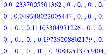
The kinetic energy matrix is diagonal, because the sine functions are eigenfunctions of the ree-particle Hamiltonian operator.

The potential energy matrix is obviously symmetric.

>	VM:=Matrix(Nb,Nb,shape=symmetric):

>	HM:=Matrix(Nb,Nb,shape=symmetric):

>	for m from 1 to Nb do: for n from 1 to m do: VM[m,n]:=int(BF(m)*V*BF(n),r=0..Rb): od: od:

>	#print(map(evalf,VM));

>	for m from 1 to Nb do: for n from 1 to m do: HM[m,n]:=evalf(VM[m,n]): if m=n then HM[m,n]:=HM[m,n]+evalf(TM[m,m]): fi: od: od:

>	convert(sort(Eigenvalues(HM)),list);

$\left[-.970436859393496686e-2,.252249064690672383e-1,.813410797023288585e-1,.163862387254931130,.272034762720016088,.405532046828107396,.564174578760980094,.747846440168513204,.956467123828828370,1.18997954958329432,1.44834383238341924,1.73153386712198021,2.03953590687572506,2.37234903560626264,2.72998788467661813,3.11248849670469285,3.51991957815230627,3.95240698551275526,4.41021078026597824,4.89415888192453340\right]$

The matrix eigenvalues are upper bounds to the true differential equation eigenvalues. We can have certainty over the accuracy of the bound part of the spectrum after performing a convergence analysis.

We seem to have only one bound state with an energy of E=-0.0097 units.

Note that matrix diagonalization results in a 'discretized continuum' of E>0 eigenenergies. These are called pseudo-continuum states, because the eigensolutions vanish at the box edge set by Rb, and are not meaningful outside of the box.

Let us generate the differential equation solution:

>	E0:=-.970436859393496686e-2;

$\mathrm{E0}:=-.970436859393496686e-2$

>	SE:=-0.5*diff(u(r),r$2)+(V-E0)*u(r)=0;

$\mathrm{SE}:=-.5\left(\frac{d^2}{{dr}^2}u\left(r\right)\right)+\left(-e^{\left(-r\right)}+.970436859393496686e-2\right)u\left(r\right)=0$

>	IC:=u(0)=0,D(u)(0)=1;

$\mathrm{IC}:=u\left(0\right)=0,\left(u^{\prime }\right)\left(0\right)=1$

>	sol:=dsolve({SE,IC},numeric,output=listprocedure):

>	uS:=eval(u(r),sol):

>

uS(1);

$.808060539074445640$

>	plot(uS(r),r=0..Rb,thickness=2);

One should do the following checks:

1) the matrix diagonalization solution is still affected by the finite value of Rb (the cut-off distance at large r); why? the numerical solution is showing a node before r=20, which means that iterating on E0 to generate a smooth approach towards the axis would yield a slightly lower E0 *ASSIGNMENT*

    one check that should be applied: what is the classical turning point for the given E and V? this is done below.

2) basis size will play a role when the real axis is extended (Rb is increased) further. The matrix diagonalization ground-state energy should converge towards the 'exact' numerical ODE solution.

3) a further check would be: does this one bound state remain the only one? When the matrix size is increased, is it possible that another E<0 solution appears (in the L=0 sector)? What if the potential constant V0=1 is increased?

ASSIGNMENT: Choose a deeper potential (either by increasing V0 or by changing the r-scaling, exp(-r) can be changed to exp(-0.5*r), etc.; such that two bound states exist for L=0. Then re-do the phase shift calculation as a function of k, and observe whether it starts at 2*pi for k=0.

The classical turning point:

>	R_tp:=solve(E0=V,r);

$4.6351791243504$

The weakly bound state has a long probability amplitude tail in the tunneling region.

Can we measure the scattering length a?

The definition according to eq. (3.3) on p.44 says that tan(delta) goes like -k*a (we can ignore the shift by pi)

>

>	kL[1],PS_L[1];

$.5e-1,-.42061561544355$

>	a_guess:=-tan(PS_L[1])/kL[1];

$\mathrm{a\_guess}:=8.9462227047440$

>	-tan(PS_L[2])/kL[2];

$9.7986571953445$

We should fit the data to make an accurate estimate:

>

k:='k';

$k:=k$

>	with(Statistics):

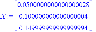
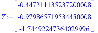
>	X := Vector([seq(kL[j],j=1..3)], datatype=float); Y := Vector([seq(tan(PS_L[j]),j=1..3)], datatype=float);

>	LinearFit([k, k^2, k^3], X, Y, k);

Warning, there are zero degrees of freedom

$-9.07551301913381180k+12.4030543376996523k^2-196.344960998065346k^3$

We need more data, and we should concentrate on lower wavenumber values!

>	kL1:=[0.01,0.02,0.03,0.04];

>	PS_L1:=PhSh(kL1);

$\mathrm{kL1}:=\left[.1e-1,.2e-1,.3e-1,.4e-1\right]$

$\mathrm{PS\_L1}:=\left[-.86812200427120e-1,-.17291166386013,-.25762640494214,-.34036020287531\right]$

>	X := Vector([seq(kL[j],j=1..4)], datatype=float); Y := Vector([seq(tan(PS_L[j]),j=1..4)], datatype=float);

>	LinearFit([k, k^2, k^3], X, Y, k);

$-10.7052884308109420k+47.4310631856857583k^2-361.755002780221957k^3$

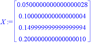
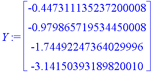
We see that the fit is far from converged! Probably a good place for an assignment question!

Theory (page 51) also points out that the tangent of the phase shift has linear plus cubic terms at lowest orders

>	LinearFit([k, k^3, k^5], X, Y, k);

$-8.85467663672005934k-63.2115197881197304k^3-2701.80843655814215k^5$

Note that the minus sign convention in the scattering length is not universal, some authors don't put it in.

Now let us check that the E=0 solution for the SE has a node at about a.

>

>	E0:=1E-10; # going for zero energy

$\mathrm{E0}:=.1e-9$

>	SE:=-0.5*diff(u(r),r$2)+(V-E0)*u(r)=0;

$\mathrm{SE}:=-.5\left(\frac{d^2}{{dr}^2}u\left(r\right)\right)+\left(-e^{\left(-r\right)}-.1e-9\right)u\left(r\right)=0$

>	IC:=u(0)=0,D(u)(0)=1;

$\mathrm{IC}:=u\left(0\right)=0,\left(u^{\prime }\right)\left(0\right)=1$

>	sol:=dsolve({SE,IC},numeric,output=listprocedure):

>	uS:=eval(u(r),sol):

>

uS(1);

$.805209497570437916$

>	plot(uS(r),r=0..2*Rb,thickness=2);

This verifies the claim that the scattering length corresponds to the first node location in the E=0 solution. Question: are there more nodes for the E=0 solution above?

>

>

>

>

>