- java.lang.Object
-
- java.awt.Component
-
- java.awt.Container
-
- java.awt.Window
-
- java.awt.Frame
-
- javax.swing.JFrame
-
- AnovaGUI
-
- All Implemented Interfaces:
- java.awt.event.ActionListener, java.awt.event.ItemListener, java.awt.image.ImageObserver, java.awt.MenuContainer, java.io.Serializable, java.util.EventListener, javax.accessibility.Accessible, javax.swing.RootPaneContainer, javax.swing.WindowConstants
public class AnovaGUI
extends javax.swing.JFrame
implements java.awt.event.ActionListener, java.awt.event.ItemListener
AnovaGUI
Summary
- A utility to perform an analysis of variance (ANOVA) on a table of data read from a file
Table of Contents
- Launch
- Designs Supported
- Arguments
- Data Organization
- Header Lines
- Examples
- One-Way With One Within-Subject Factor (W)
- Two-Way With One Within-Subjects Factor And One Between-Subjects Factor (W-B)
- Two-Way With Two Within-Subjects Factors (W-W)
- Three-Way With Two Within-Subjects Factors And One Between-Subjects Factor (W-W-B)
- One-Way With One Between-Subjects Factor (B)
- Multiple Between-subjects Factors (B-B, B-B-B)
- Additional Designs
- Effect Sizes
- Missing Data
Launching AnovaGUI
Launch AnovaGUI from GoStats as follows: (click to enlarge)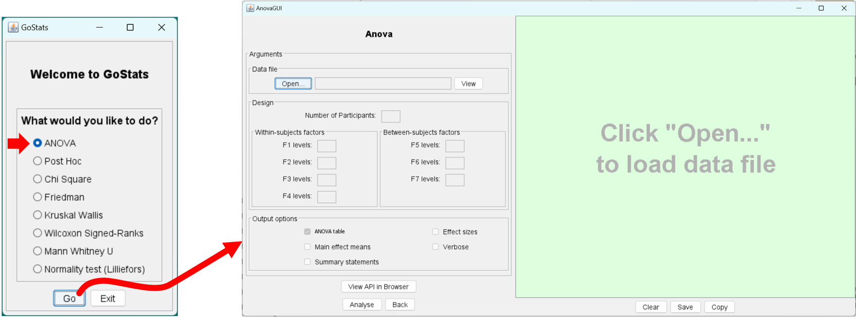
Designs Supported
Sixteen experiment designs are supported:Design Factors Summary W F1 One-way with one within-subjects factor (Example) W-W F1, F2 Two-way with two within-subjects factors (Example) W-W-W F1, F2, F3 Three-way with three within-subjects factors W-W-W-W F1, F2, F3, F4 Four-way with four within-subjects factors B F5 One-way with one between-subjects factor (Example) B-B F5, F6 Two-way with two between-subjects factors (Example) B-B-B F5, F6, F7 Three-way with three between-subjects factors W-B F1 | F5 Two-way mixed design with one within-subjects factor and one between-subjects factor (Example) W-B-B F1 | F5, F6 Three-way mixed design with one within-subjects factor and two between-subjects factors W-B-B-B F1 | F5, F6, F7 Four-way mixed design with one within-subjects factor and three between-subjects factors W-W-B F1, F2 | F5 Three-way mixed design with two within-subjects factors and one between-subjects factor ( Example) W-W-B-B F1, F2 | F5, F6 Four-way mixed design with two within-subjects factors and two between-subjects factors W-W-B-B-B F1, F2 | F5, F6, F7 Five-way mixed design with two within-subjects factors and three between-subjects factors W-W-W-B F1, F2, F3 | F5 Four-way mixed design with three within-subjects factors and one between-subjects factor W-W-W-B-B F1, F2, F3 | F5, F6 Five-way mixed design with three within-subjects factors and two between-subjects factors W-W-W-W-B F1, F2, F3, F4 | F5 Five-way mixed design with four within-subjects factors and one between-subjects factors Note on terminology: A factor is often called an independent variable. The levels of a factor are often called test conditions or, in statistics textbooks, treatments. A within-subjects factor is often called a repeated-measures factor.
Arguments
AnovaGUI works with 14 arguments, consisting of nine text fields and five checkboxes:
Argument input is disabled until a data file is opened for analysis. If the data file includes header lines (see below), the values of arguments are automatically determined.
The arguments are now described.
Argument Description Data file The file containing the data. See below for the required organization of the data file. Number of participants The number of participants represented in the data file. This argument is automatically determined when the data file is opened. The number of participants is the number of rows of data in the data file. Within-subjects factors F1 Number of levels of the first within-subjects factor, if any. This argument is automatically determined when the data file is opened, if the data file has header lines (see below). This argument is only required if the experiment has at least one within-subjects factor.
F2 Number of levels of the second within-subjects factor, if any. This argument is automatically determined when the data file is opened, if the data file has header lines (see below). This argument is only required if the experiment has at least two within-subjects factors.
F3 Number of levels of the third within-subjects factor, if any. This argument is automatically determined when the data file is opened, if the data file has header lines (see below). This argument is only required if the experiment has at least three within-subjects factors.
F4 Number of levels of the fourth within-subjects factor, if any. This argument is automatically determined when the data file is opened, if the data file has header lines (see below). This argument is only required if the experiment has four within-subjects factors.
Between-subjects factors F5 Number of levels of the first between-subjects factor, if any. This argument is automatically determined when the data file is opened, if the data file has header lines (see below). This argument is only required if the experiment has at least one between-subjects factor.
F6 Number of levels of the second between-subjects factor, if any. This argument is automatically determined when the data file is opened, if the data file has header lines (see below). This argument is only required if the experiment has at least two between-subjects factors.
F7 Number of levels of the third between-subjects factor, if any. This argument is automatically determined when the data file is opened, if the data file has header lines (see below). This argument is only required if the experiment has three between-subjects factors.
Output options ANOVA table A checkbox output argument. If selected, this option produces the ANOVA table when the Analyse button is clicked. Main effect means A checkbox output argument. If selected, this option outputs the main effect means and the participant means. The main effect means are the means for the levels of an independent variable. Examining and comparing the means for the participants and test conditions is important in experimental research. However, this option is also useful to ensure that the data are properly organized for designs with more than one within-subjects or between subjects independent variable. For example, if the data are improperly nested for a two-factor design, this will be apparent by comparing the output from this option against a manual or spreadsheet calculation of the effect means.
Summary statements A checkbox output argument. If selected, this option outputs generic statements giving the results of the ANOVA. Statements are provided for the main effects and the two-way interaction effects. The relevant statistics are pulled from the ANOVA table and presented in the usual manner in parentheses at the end of each statement. Effect sizes A checkbox output argument. If selected, this option outputs the effect sizes for all main effects and two-way interactions. The output includes partial eta squared (ηp2) and omega squared (ω 2). Verbose A checkbox output argument. If selected, this option outputs additional information, including the original data, the sorted data, the means by participant and condition, the sums of squares, the mean squares, the degrees of freedom, the F statistics, and p for the F statistics. Data Organization
The 1st argument in AnovaGUI is the data file. The data are organized in a p × n table, with p rows and n columns. Values are space- or comma-delimited. p is the number of participants and n is the number of within-subjects test conditions plus the number of between-subjects factors.The number of participants (p) is the number of rows of data and appears as the 2nd argument.
The number of within-subjects test conditions, if any, is derived from the 3rd, 4th, 5th, and 6th arguments. These arguments are the number of levels of the F1, F2, F3, and F4 within-subjects factors. The number of between-subjects factors, if any, is the number of additional columns which contain group codes for between-subjects factors.
The following is a simple example for an experiment with 12 participants and one within-subjects factor (F1) with three levels (L1, L2, L3).
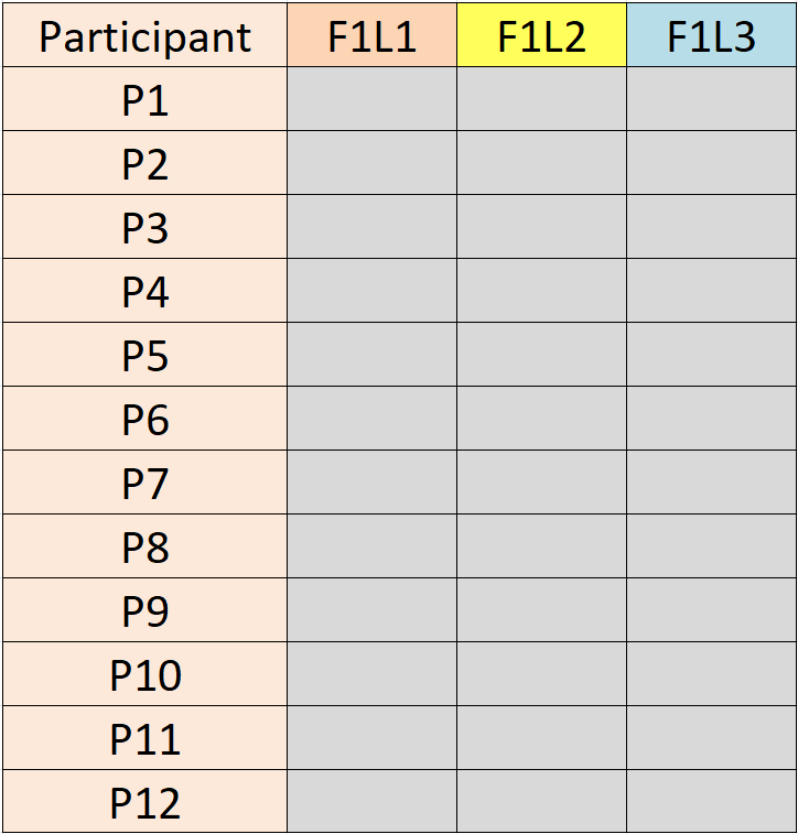
Only the data (grey cells) are in the data file. Each data entry is a measurement on the dependent variable. The dependent variable is the human behaviour of interest, such as task completion time in seconds.
The test conditions for a within-subjects factor are often presented to participants in a counterbalanced order to offset learning effects. Typically, the order is determined by a Latin square. For three test conditions, A, B, and C, there are three orders: ABC, BCA, and CAB. Participants are divided into three groups and each group is assigned the test conditions in the designated order:
- G1 = ABC
- G2 = BCA
- G3 = CAB
The researcher might want to identify the groups in the data file and verify that counterbalancing worked. To do this, "group" is added as an additional column of nominal data and effectively becomes F5, a between-subjects factor. If there are 12 participants, each group has four participants. See below.
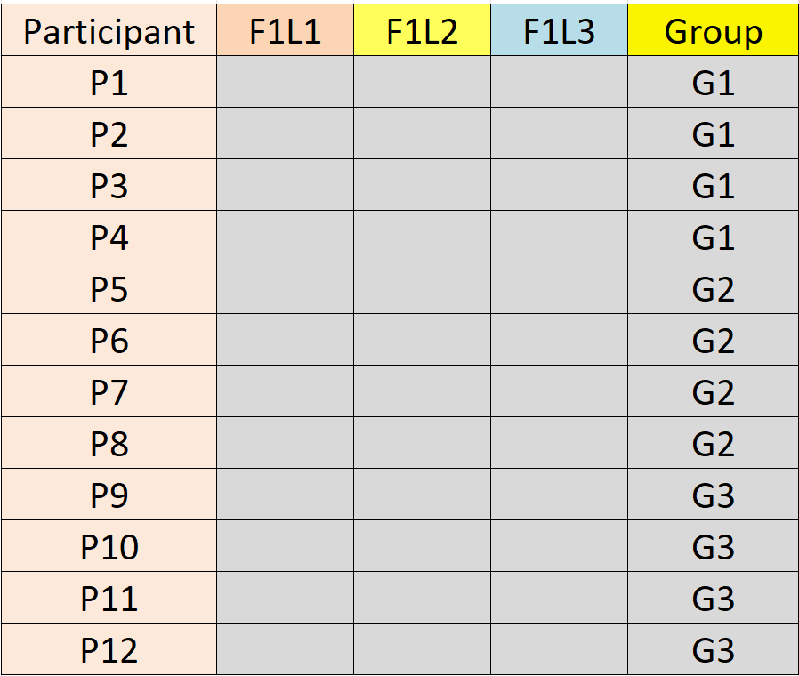
The number of levels of the between-subjects factor (three for the example above) is the value of the F5 argument.
A between-subjects factor could also identify other group circumstances, depending on the research. For example, "M" and "F" might identify male and female participants in a study on gender differences. "LH" and "RH" might identify the groups when comparing left-handed and right-handed participants. If a between-subjects factor is used, the same number of participants is required in each group. If F5 is the only factor, then the data file contains just two columns, one for the F5 data (i.e., the measurements on the dependent variable) and one for the labels that identify the F5 groups. See below.
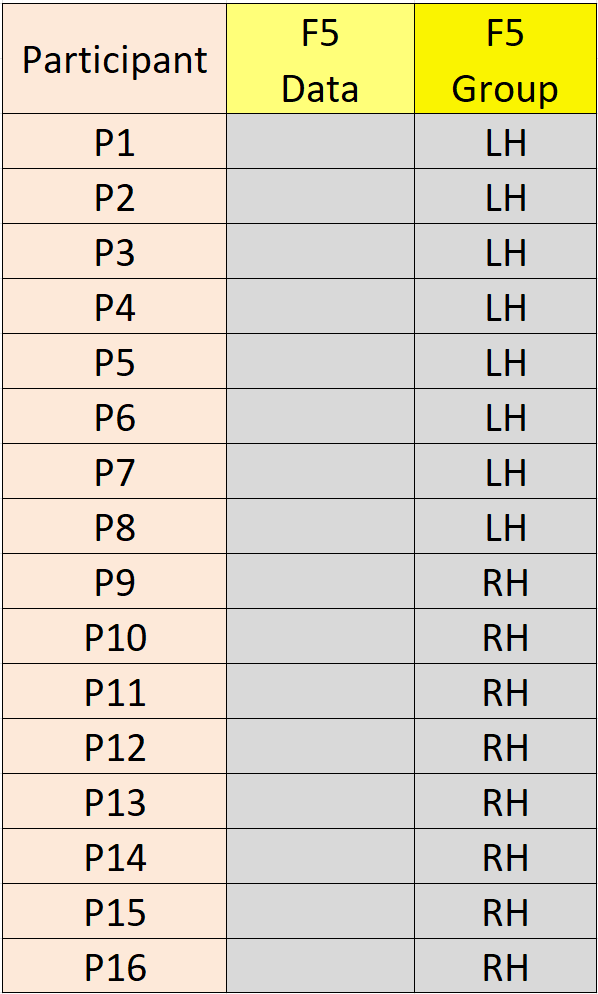
Above, the data for each group are in consecutive rows. This is not a requirement, however. If there is a between-subjects factor, the data are sorted by the between-subjects group codes before performing the ANOVA. (Note: Participant #1 corresponds to the first row in the sorted data. This point is only relevant when outputting the main effect means.)
An experiment with two within-subjects factors will have data for all combinations of the F1 and F2 factors. In this case, the data table has n1 × n2 = n columns where n 1 is the number of F1 levels and n2 is the number of F2 levels. It is important to organize the data with the levels of F2 nested inside the levels of F1. See below.
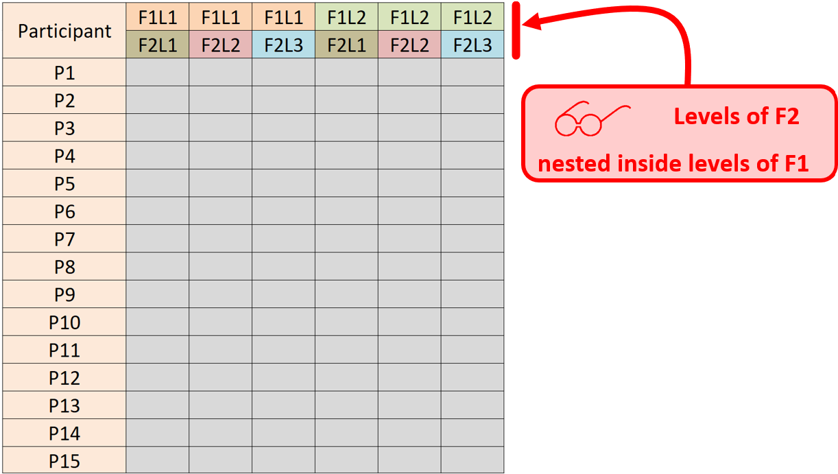
The example above is for a 2 × 3 within-subjects design. F1 has two levels and F2 has three levels. Look carefully! This point is important. If the nesting of the data do not comport with the F1 and F2 values, the ANOVA results will be meaningless.
Header Lines
AnovaGUI works in two ways, depending on whether the data file has header lines.If the data file does not have header lines, you must enter the number of levels of the factors in text fields. Also, generic labels are assigned as the names of the factors and the levels of the factors (e.g., factor "F1" with levels "L1", "L2", etc.).
If the data file has header lines, AnovaGUI automatically determines the number of levels of all factors. As well, the names of the factors and the names of the levels of the factors are automatically extracted from the header lines. Obviously, including header lines is the preferred option.
Doing an ANOVA on a data file with header lines is a simple two-step process:
- Click "Open..." to load the data file (which contains header lines).
- Click "Analyse".
Of course, you must edit the data file in advance and add the header lines.
To add header lines, insert eight lines at the beginning of the data file, formatted as follows:
     DV: dependent_variable_name
     F1: f1_name, f1_level1_name, f1_level2_name, ...
     F2: f2_name, f2_level1_name, f2_level2_name, ...
     F3: f3_name, f3_level1_name, f3_level2_name, ...
     F4: f4_name, f4_level1_name, f4_level2_name, ...
     F5: f5_name
     F6: f6_name
     F7: f7_name
Click here to see a typical data file with header lines.For the within-subjects factors, F1, F2, F3, and F4, the first entry is the name of the factor. The remaining entries (comma-delimited) are the names of the levels of the factor. As noted earlier, the levels of a factor are the test conditions. Implicitly, the number of level names is the number of levels of the factor.
For the between-subjects factors, F5, F6, and F7, only the name of the factor is provided. The names of the levels are extracted from the right-hand column(s) in the data file, which hold the group codes for between-subjects factors.
If a factor is not present, use a period ("
.") in lieu of the factor's name.***** Examples for common experiment designs follow. The examples include data sets with and without header lines.
For comparison, each analysis is also shown using a commercial statistics package called StatView (now JMP; http://www.jmp.com/).
One-Way With One Within-Subjects Factor (W)
The file
dix-example-10x2.txtis found in the GoStatsExamples directory that was created when GoStats was launched for the first time. The file contains656,702 259,339 612,658 609,645 1049,1129 1135,1179 542,604 495,551 905,893 715,803The data are from an example in Dix et al.'s Human-Computer Interaction (Prentice Hall, 2004, 3rd ed., p. 337). The single within-subjects factor (F1) is icon design with two levels, natural and abstract. The data are the measurements on the dependent variable, task completion time (in seconds). This was the time to name the icons in an identification task. The first column holds the measurements for the natural icons, while the second column holds the measurements for the abstract icons. Each row contains the measurements for one participant. The experiment used 10 participants.To load the file, click "Open...", choose the GoStatsExamples directory and select
dix-example-10x2.txt. The file is read with the contents shown in the right-side panel in AnovaGUI: (click to enlarge)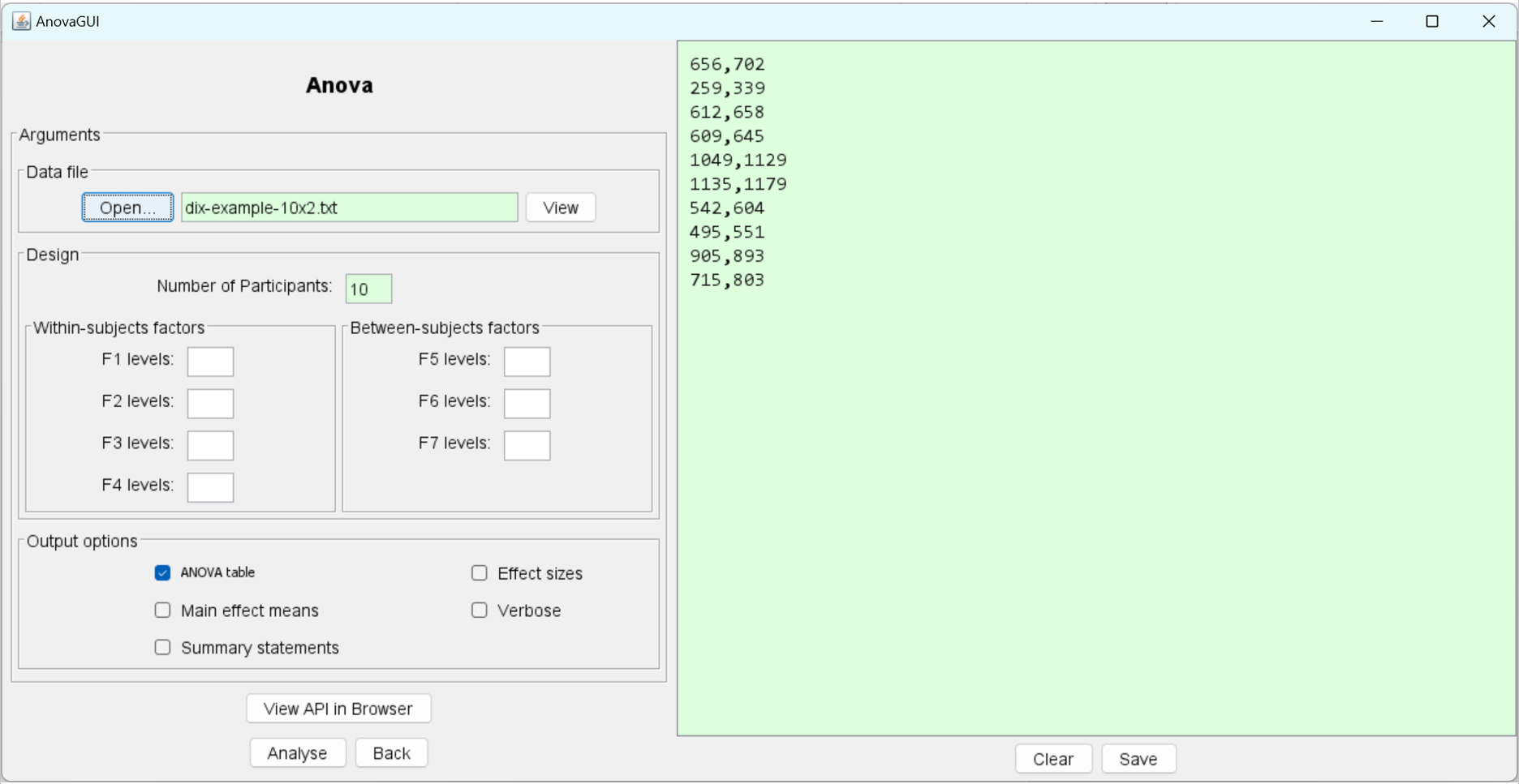
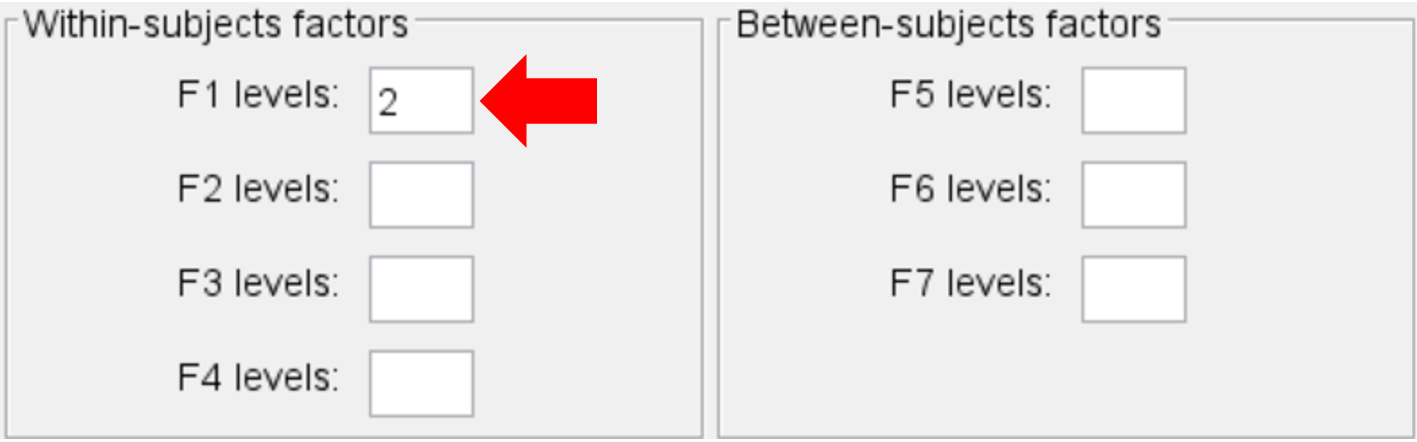
The name of the data file and the number of participants appear in text fields. The green background indicates that editing is disabled in the field. The number of participants is automatically determined by the number of rows of data in the file. However, the file does not contain header lines, so the design of the experiment is unknown. In this case, values must be entered in the Fn text fields, as appropriate. For this example, there is one factor, F1, with two levels. So, "2" is typed into the F1 field:
Before doing the ANOVA, it is useful to examine the data and compute the means for each participant and for each test condition. This done using the output option for "Main effect means":
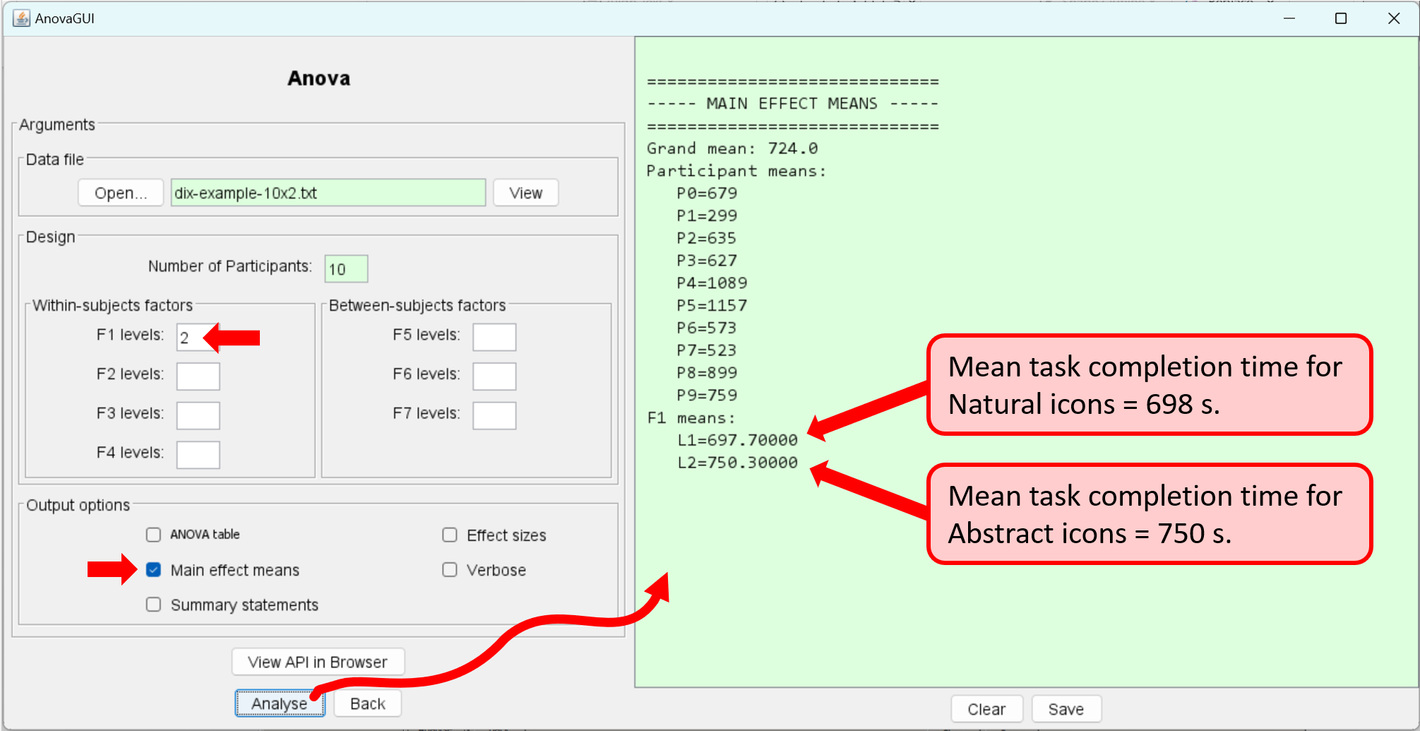
The mean task completion times were 698 s for the natural icons and 750 s for the abstract icons. The issue we are seeking to resolve is whether the difference in the means is real or is due to chance. For this, we use AnovaGUI.
The analysis of variance tests the null hypothesis that there is no significant difference between the means. The analysis is performed as follows:
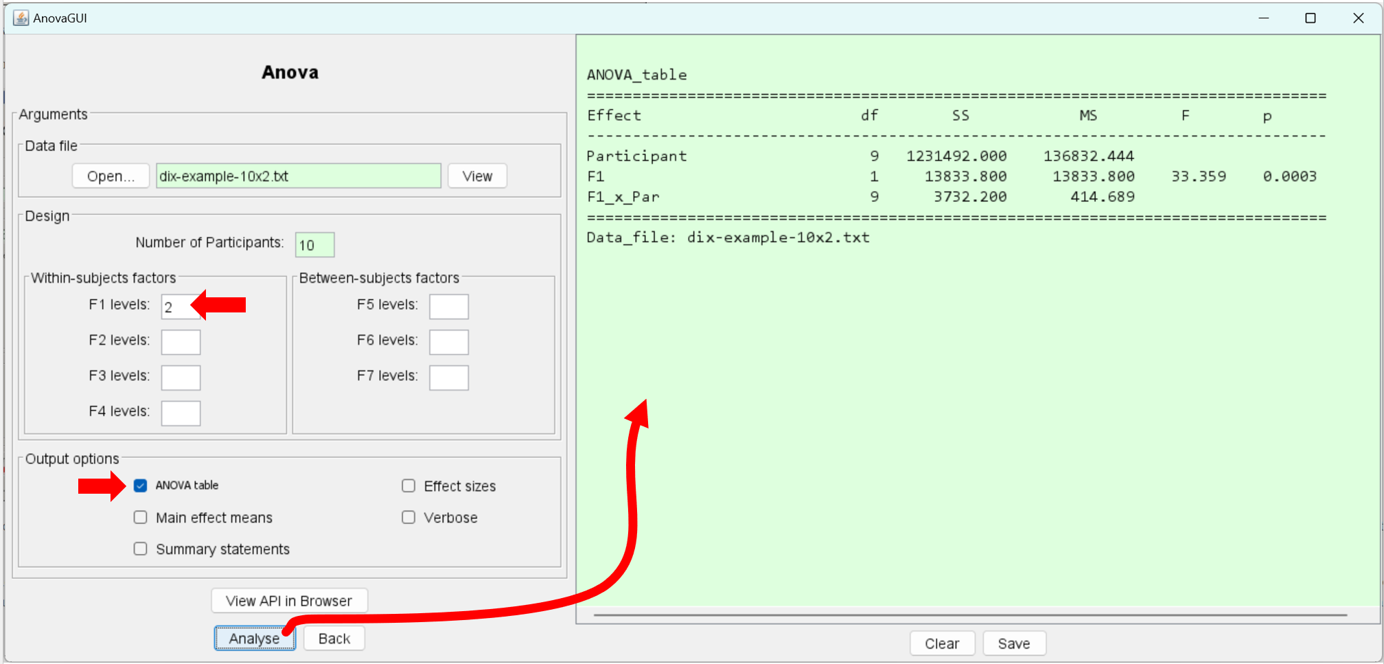
The F-statistic is 33.359. This is computed by dividing the mean squares for the F1 effect by the residual mean squares: F = MS F1 / MSF1_x_Par = 13833.8 / 414.689 = 33.359. The effect and residual degrees of freedom are 1 and 9, respectively. Consult a statistics reference for full details on the calculations. A recommended source is D. J. Sheskin's Handbook of Parametric and Non-parametric Statistical Procedures (5th edition, CRC Press, 2011).
The most important statistic in the ANOVA table is p, for probability. This is the probability of obtaining the observed data if the null hypothesis is true. If p < .05, there is less than a 1-in-20 chance we would have obtained the observed data if the null hypothesis is true. By convention, this is the threshold for significance. If p < .05, the null hypothesis of "no difference" is rejected. The conclusion is that there is a difference in the means and it is statistically significant. For the ANOVA above, p = .0003; so, indeed, the difference in the means is significant. The ANOVA result might be summarized in a research paper as follows:
The effect of icon type on task completion time was statistically significant (F 1,9 = 33.36, p < .0005). In fact, AnovaGUI will output statements as above if the output option "Summary statements" is selected.
Even though p = .0003 in the table, it is typically reported in research papers as p < n, where n is the closest more conservative value from the set .05, .01, .005, .001, .0005, and .0001. The following illustrates for the current example:
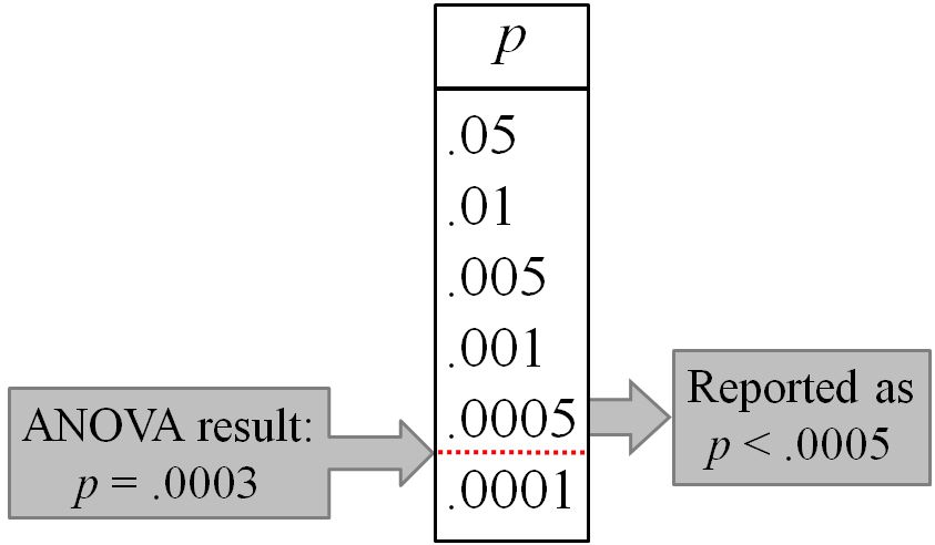
Although less common, it is also acceptable to report the exact value of p.
The difference in the means is considered not significant if p > .05. This implies there is a 5% or greater chance that the observed data would arise if the null hypothesis is true. By convention, this is sufficient uncertainty to deem the null hypothesis tenable. In other words, the null hypothesis of no difference is retained.
There are two ways to report probability for a non-significant outcome, depending on the value of F:
- If p > .05 and F > 1, report as "p > .05"
- If p > .05 and F ≤ 1, report as "ns" (for "not significant")
The latter style is used because it is impossible for differences in the means to be significant if F ≤ 1.
The results above are shown below in an ANOVA on the same data using StatView.
Lambda and Power are not reported in AnovaGUI. Lambda is a measure of the noncentrality of the F distribution, calculated as F × N, where N is the degrees of freedom of the effect. Power, which ranges from 0 to 1, is the ability to detect an effect, if there is one. The closer to one, the more the experiment is likely to find an effect, if one exists in the population. Power > .80 is generally considered acceptable; i.e., if p is significant and Power > .80, then it is likely that the effect found actually exists.
Two-Way With One Within-Subjects Factor And One Between-Subjects Factor (W-B)
The experiment described by Dix et al. (see above) used a within-subjects design. In most cases, the experiment would also use counterbalancing to offset learning effects as participants proceed from one test condition to the next. Let's explore this idea.
With two conditions, participants are divided into two groups of equal size. Half are tested on the natural icons first followed by the abstract icons, while the other half are tested in the reverse order. Like this, "group" is a between-subjects factor with five participants in each group. To include this in the analysis, we add a column to the data file, creating a new data file called
dix-example-h10x2b.txt. The new column identifies the groups as either "NA" (natural first, abstract second) or "AN" (abstract first, natural second). The file is also modified to include header lines, as per the requirements noted above. Here are the data:DV: Completion Time (s) F1: Icon Type, Natural, Abstract F2: . F3: . F4: . F5: Group F6: . F7: . 656,702,NA 259,339,NA 612,658,NA 609,645,NA 1049,1129,NA 1135,1179,AN 542,604,AN 495,551,AN 905,893,AN 715,803,ANThe file is loaded, as before: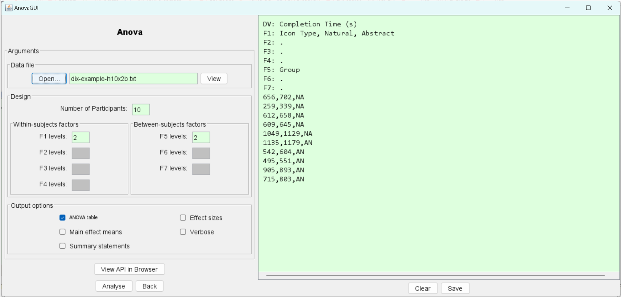
The header lines provide enough information for AnovaGUI to determine which factors are included and the number of levels of each. In the image above, note that the within-subjects factor F1 is present with two levels and the between-subjects factor F5 is present with two levels. F2, F3, F4, F6, and F7 are not used, so the corresponding text fields are disabled.
After clearing the right-side panel by clicking "Clear", we click "Analyse":
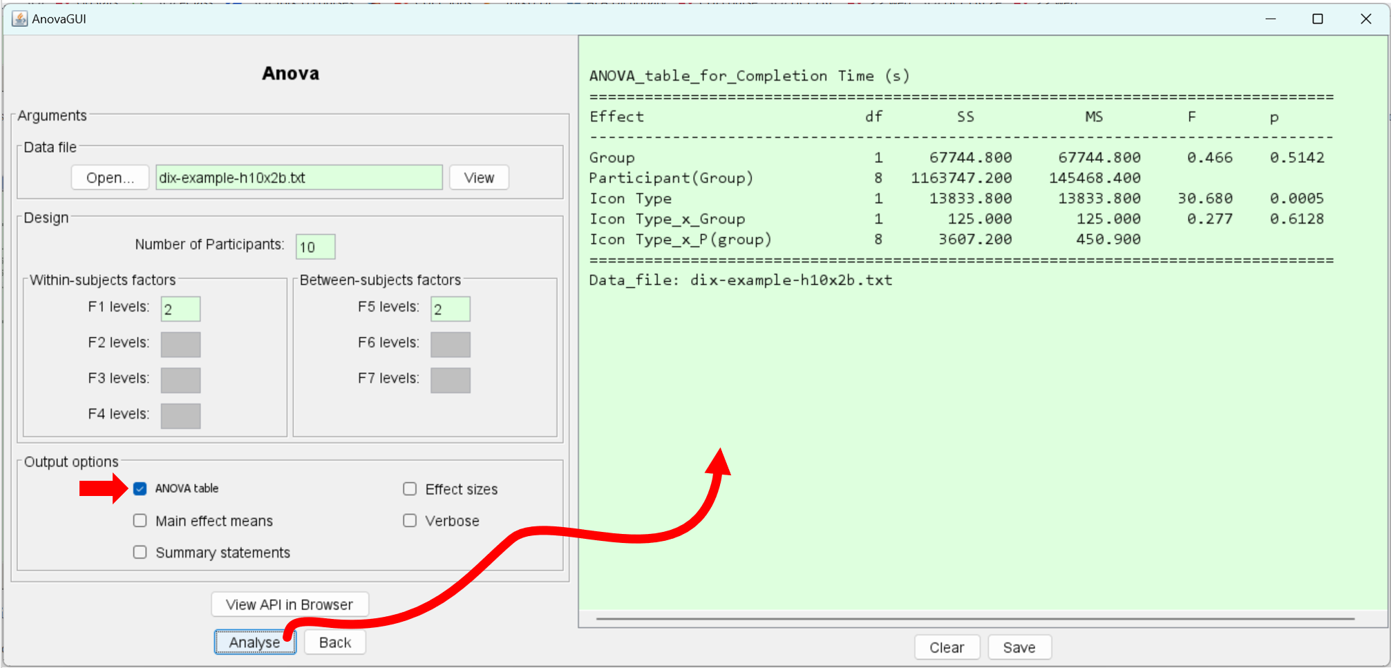
Note that the ANOVA table now includes the name of the dependent variable, Completion Time (s), and the names of the independent variables, Icon Type and Group. These were extracted from the header lines in the data file.
The group effect (see above) was not statistically significant (F1,8 = 0.466, ns). This is good news, since it means counterbalancing worked. Any learning effect that might have occurred for the AN group was effectively offset by an opposing learning effect for the NA group.
The F and p statistics for the effect of icon type (see above) are slightly different than the earlier test which did not include group. This is simply an artifact of how the variances are partitioned when the group factor is added in the analysis. However, the outcome is the same: There is a significant effect of icon type on task completion time (F1,8 = 30.68, p < .0005).
The same analysis in StatView appears as
Two-Way With Two Within-Subjects Factors (W-W)
Consider an experiment on "face input" – using a smart phone's front-facing camera to track face movement as an input modality. The experimental methodology and data analyses for this example are described in FittsFace: Exploring navigation and selection methods for facial tracking (Cuaresma & MacKenzie, HCII 2017). The experiment was a 2 × 3 repeated-measures design with 12 participants. The factors and levels were as follows:
Factor Levels Navigation method Positional, Rotational Selection method Smile, Blink, Dwell Counterbalancing was used but this is not considered here.
The task was a Fitts' law target selection task, as commonly used in experiments comparing input methods. Two face-tracking navigation methods were tested, and for each navigation method, three selection methods were tested. Although there were several dependent variables, only throughput (bps) is presented here. The data are in
throughput-h12x6.txt:DV: Throughput (bps) F1: Navigation method, Positional, Rotational F2: Selection method, Smile, Blink, Dwell F3: . F4: . F5: . F6: . F7: . 0.555 0.546 0.433 0.506 0.360 0.137 0.472 0.621 0.376 0.655 0.519 0.407 0.692 0.505 0.613 0.375 0.466 0.157 0.743 0.712 0.621 0.594 0.361 0.488 0.677 0.603 0.535 0.438 0.262 0.282 0.636 0.618 0.603 0.401 0.200 0.328 0.461 0.652 0.413 0.440 0.409 0.254 0.634 0.642 0.601 0.400 0.547 0.453 0.517 0.513 0.429 0.328 0.064 0.092 0.493 0.433 0.477 0.413 0.400 0.188 0.588 0.522 0.609 0.381 0.231 0.385 0.785 0.708 0.688 0.409 0.259 0.462Eight header lines were manually inserted to improve the output and simplify the analysis.The output option "Main effect means" is used prior to the analysis, to view the overall effect means:
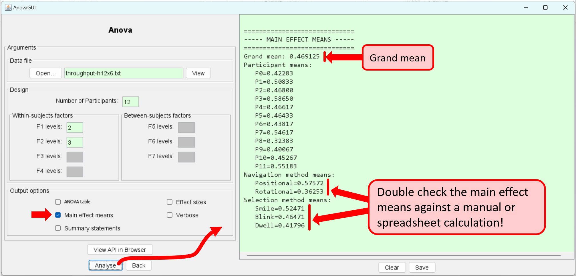
As seen above, the grand mean for throughput was 0.47 bps. This is low compared to values reported in other experiments for devices such as the computer mouse. By navigation method, the means were 0.36 bps for rotational navigation and 0.58 bps for positional navigation, the latter being about 60% higher. The throughputs for the three selection methods were 0.52 bps (smile), 0.46 bps (blink), and 0.42 bps (dwell).
Examining the main effect means, as above, is highly recommended for designs with two or more within-subjects factors. The objective is to ensure that the data are correctly organized with the levels of the F2 factor nested inside the levels of the F1 factor, as noted earlier. As well, the data columns and the levels of the factors are ordered left-to-right. So, for this example, the positional and rotational data for F1 are in columns 1-3 and 4-6, respectively, while the smile, blink, and dwell data for F2 are in columns 1 & 4, 2 & 5, and 3 & 6, respectively.
The analysis of variance is performed as follows:
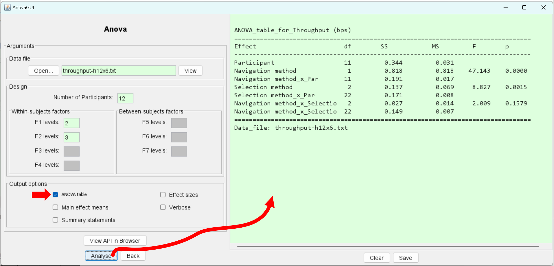
As shown, the main effect of navigation method on throughput was statistically significant (F1,11 = 47.1, p < .0001). There was also a significant effect of selection method on throughput ( F 2,22 = 8.83, p < .005). However, the Navigation Method × Selection Method interaction effect was not significant (F2,22 = 2.01, p > .05).
The same data analysed in StatView yield the following ANOVA table:
Three-Way With Two Within-Subjects Factors And One Between-Subjects Factor (W-W-B)
The file
softkeyboard-h12x10b.txtcontains data from an experiment comparing two layouts of soft keyboards. Participants entered the phrase "the quick brown fox jumps over the lazy dog" five times on each layout. Each entry of a phrase is called a trial. The dependent variable was entry speed in words per minute.The experiment used 12 participants in a 2 × 5 within-subjects design with the following factors and levels:
Factor Levels Layout Opti, Qwerty Trial T1, T2, T3, T4, T5 Testing was counterbalanced. Each participant entered the phrase five times with one layout, then five times with the other layout. Half the participants first used Opti (A), following by Qwerty (B). The other half used the layouts in the reverse order. Thus, group is added as a between-subjects factor with two levels, coded as "AB" and "BA".
Since group – the between-subjects factor for counterbalancing – is of no particular interest in the research, it is commonly omitted when summarizing the design of the experiment, as above.
The data file was edited to add the variable names in header lines and the participant group as the last entry on each data line: (abbreviated to fit page)
     DV: Entry Speed (wpm)
     F1: Layout, Opti, Qwerty
     F2: Trial, T1, T2, T3, T4, T5
     F3: .
     F4: .
     F5: Group
     F6: .
     F7: .
     7.589351375,12.37706884, ... 31.34872418,31.55963303,33.81389253,AB
     9.32417781,12.900000000, ... 28.89137738,29.94776553,35.0305499,AB
     9.207708779,9.504512802, ... 24.14599906,27.95232936,28.10457516,AB
     7.158712542,7.754733995, ... 25.0242483,20.65652522,24.80769231,AB
     9.532606688,13.18007663, ... 28.58725762,30.75089392,30.55062167,AB
     9.290601368,11.66628985, ... 26.9733403,24.71264368,28.74651811,AB
     9.417776967,9.194583036, ... 27.21518987,28.04347826,28.32052689,BA
     5.347150259,7.188631931, ... 20.31496063,19.28971963,20.39525692,BA
     14.1797197,15.10980966,  ... 30.71428571,31.67587477,34.01450231,BA
     8.970792768,10.39693734, ... 27.68240343,25.51928783,25.12171373,BA
     9.552017771,12.69372694, ... 30.97238896,32.33082707,33.7254902,BA
     8.510638298,12.11267606, ... 33.07692308,32.84532145,32.04968944,BA
The main effect means are computed as follows: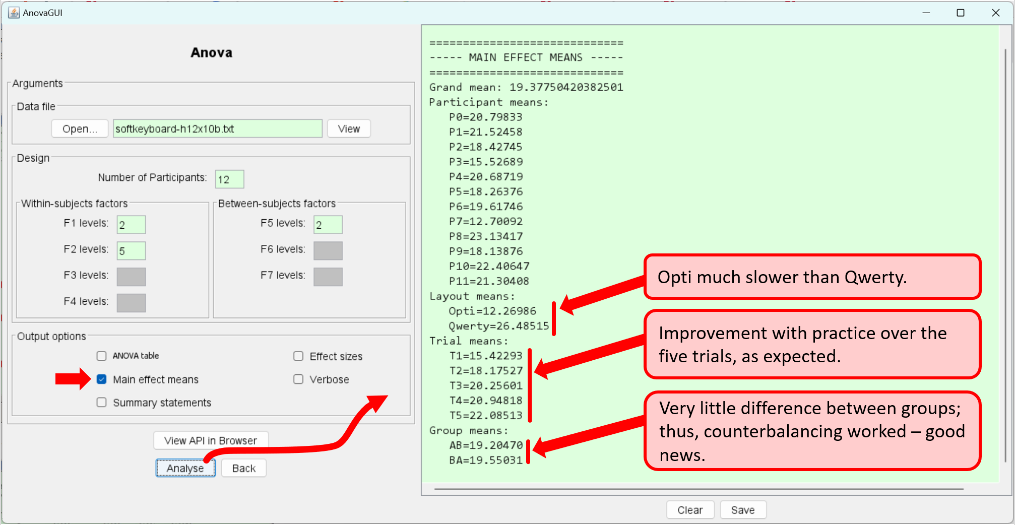
Entry speed in words per minute was much faster with the Qwerty layout (26.5 wpm) than with the Opti layout (12.3 wpm). Let's see if the difference in the means is statistically significant:
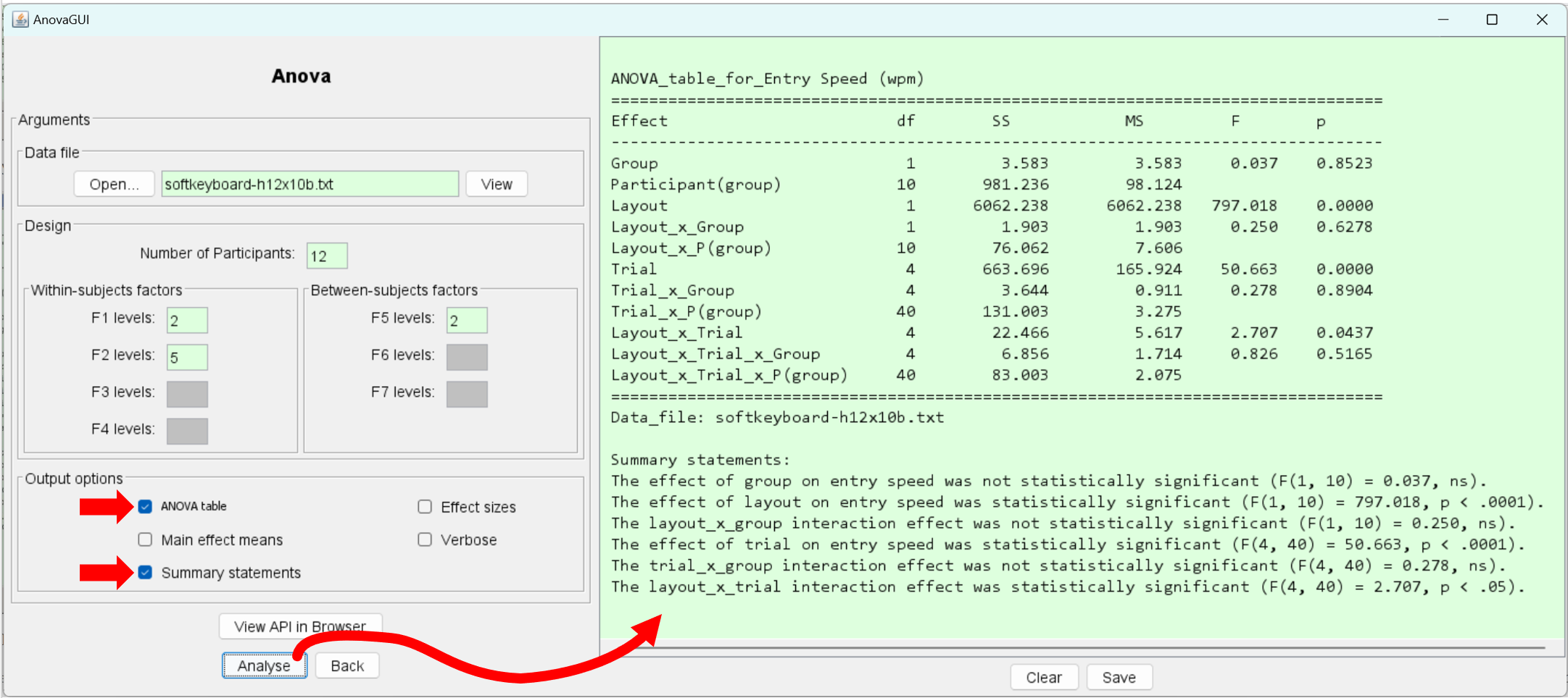
Yes. The F statistic for the layout effect is 797.0, which is extremely high. Not surprisingly, the main effect of layout on entry speed is highly significant (F1,10 = 797.0, p < .0001). In all, the table shows three main effects and four interaction effects.
Generic summary statements appear above, as provided using the "Summary statements" output option. Of course, there is considerable leeway in presenting the results in a research paper. See Experiment 1 in "Using Paper Mockups for Evaluating Soft Keyboard Layouts" (MacKenzie & Read, CASCON 2007) for an example of how results like these might be reported.
When formatting the ANOVA results in a research paper, there are two accepted styles. Examples for the last summary statement above are given below.
The ANOVA results above are confirmed using StatView:
One-Way With One Between-Subjects Factor (B)
A one-way between-subjects design might be used, for example, to test whether an interface or interaction technique works better with left-handed or right-handed users (or with males or females). In this case, the design must be between-subjects because a participant cannot be both left-handed and right-handed (or male and female!). Two groups of participants are required. Let's consider the case where five left-handed users and five right-handed users are measured on a task. The independent variable is handedness with two levels, left-handed (LH) and right-handed (RH), and the dependent variable is the time to complete a task (in seconds). Here are the example data, stored in
anova-h10b.txt:DV: Time (s) F1: . F2: . F3: . F4: . F5: Handedness F6: . F7: . 25.6,LH 23.4,LH 19.4,LH 28.1,LH 25.9,LH 14.3,RH 22.0,RH 30.4,RH 21.1,RH 19.3,RHThe means (not shown) for the LH and RH groups were 24.5 s and 21.4 s, respectively. Evidently, the left-handed group took about 14% longer to complete the task. That's a considerable performance difference, but is the difference in the means statistically significant? Let's find out: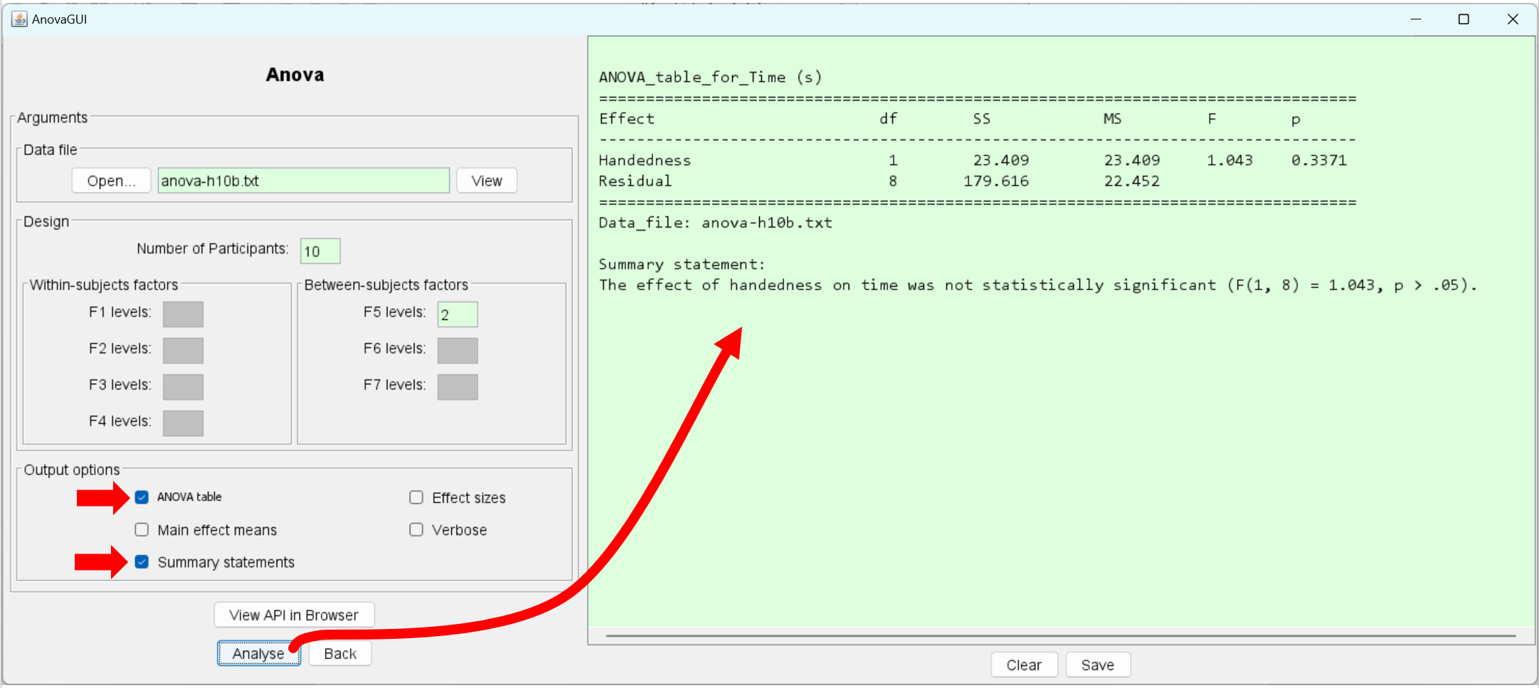
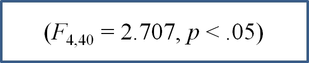
No. Despite the observation that the left-handed group took longer to complete the task, the difference between the groups was not statistically significant (F1,8 = 1.04, p > .05). This might be due to the small number of participants tested. It might also be due to a lack of bias in the interface for left-handed vs. right-handed users. We don't know.
Using StatView, the above results are confirmed:
Multiple Between-subjects Factors (B-B, B-B-B)
AnovaGUI supports up to three between-subjects factors: F5, F6, and F7. Testing must include every combination of the levels of all factors. This is the essence of a factorial experiment. As a simple example, consider an experiment with 12 participants using a 2 × 3 between-subjects design. The F5 factor has two levels or groups and the F6 factor has three levels or groups. For the F5 factor, there are 12 / 2 = 6 participants per group, and for the F6 factor, there are 12 / 3 = 4 participants per group. Furthermore, the F5-F6 combinations must be fully crossed, which is to say, the F6 factor has three groups of 2 participants in each of the groups of 6 for the F5 factor. Although the nesting requirement must be met and appropriate codes must appear in the right-hand columns, the data needn't be sorted. AnovaGUI takes care of that.The (unsorted) data for the example just described are in the file
data12x1bb.txt:302,A,X 139,A,X 551,B,X 893,B,Y 803,B,Y 222,B,Z 122,B,Z 258,A,Y 445,A,Y 129,A,Z 179,A,Z 604,B,XThe analysis proceeds as follows:
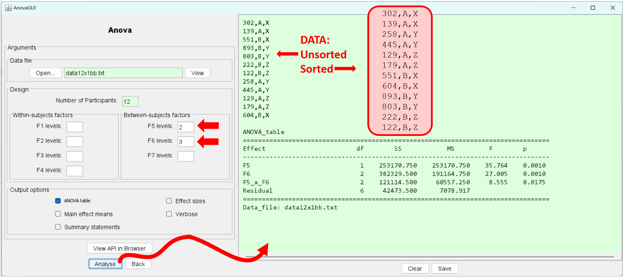
The raw data are unsorted. If between-subjects factors are present, AnovaGUI sorts the data by F5, then F6 (if present), then F7 (if present). This is shown in the highlighted data (above). The sorted data may be viewed directly using the output option "Verbose".
Additional Designs
The examples above cover the most common designs for experiments with human participants (frequently called user studies). Examples are not included for designs using three or four within-subjects factors or three between-subjects factors. We'll leave it to you to explore these possibilities.Effect Sizes
AnovaGUI includes a checkbox item to output the effect sizes for the main effects and the two-way interaction effects. As an example, let's revisit the Dix example. The image below shows the ANOVA result as well as the effect sizes.
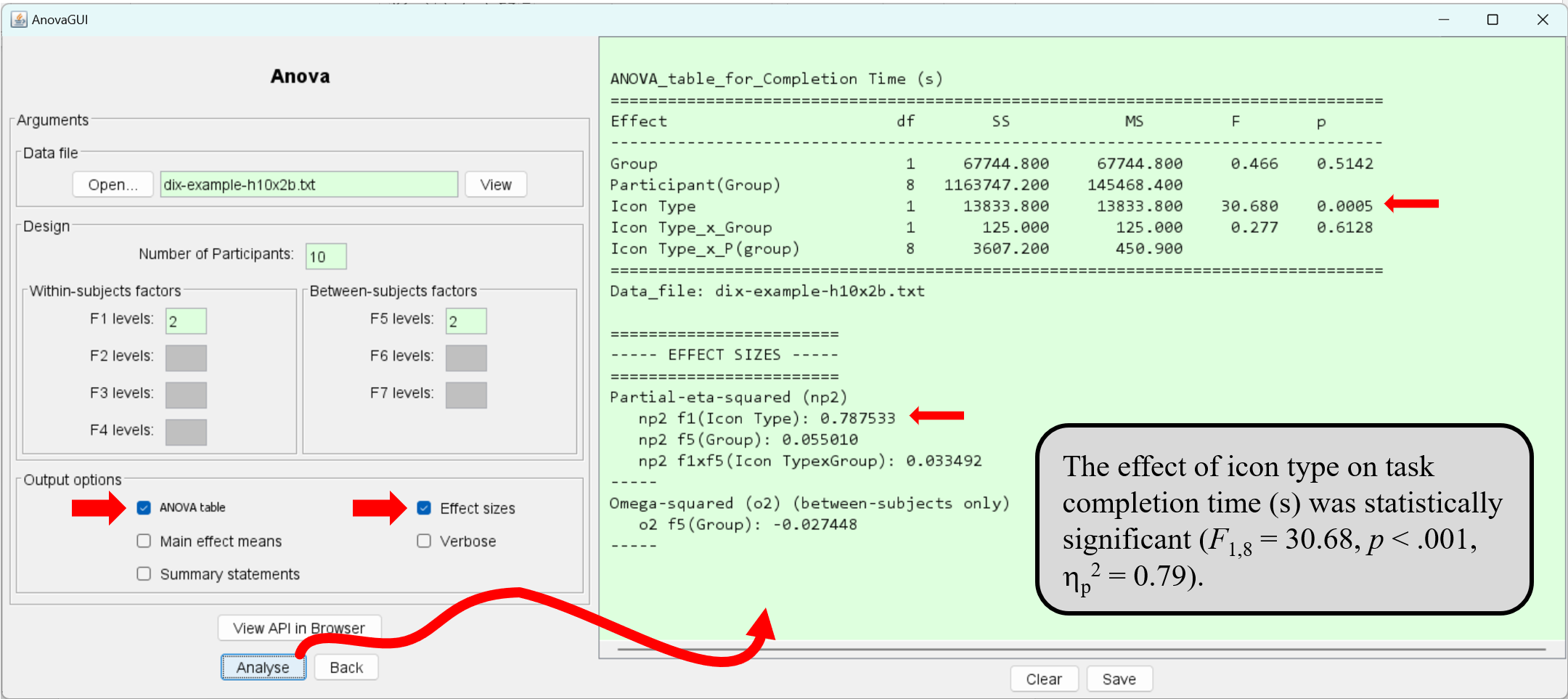
The effect size calculation is for partial eta squared, a popular effect-size metric, in part due to its inclusion in ANOVA analyses provided by SPSS. The image above includes a statement of the results of the ANOVA, including the effect size, as might appear in a research paper.
Missing Data
Although not recommended, it is possible to use AnovaGUI on data sets with missing values. Any data value missing must appear in the data file as a hash symbol ("#").There are many approaches to handling missing data. The approach here is to substitute the grand mean for each missing value. This is the most conservative approach. Variance is reduced, as is the statistical power of the test. But, the ANOVA test can proceed. Good luck.
If any data are missing, the ANOVA table will indicate the number of missing values in the footer line below the table.
-----------------------------------------------------
A note on the calculations:
The trickiest calculation is for p, representing the significance of F. This comes by way of the methodFProbabilityin theStatisticsclass in the University of Waikato'sweka.corepackage. This package was obtained fromhttp://www .cs.waikato.ac.nz/ml/weka/index.html Statistics.classcopyright notice:-----
Class implementing some distributions, tests, etc. The code is mostly adapted from the CERN Jet Java libraries: Copyright 2001 University of Waikato Copyright 1999 CERN - European Organization for Nuclear Research. Permission to use, copy, modify, distribute and sell this software and its documentation for any purpose is hereby granted without fee, provided that the above copyright notice appears in all copies and that both that copyright notice and this permission notice appear in supporting documentation. CERN and the University of Waikato make no representations about the suitability of this software for any purpose. It is provided "as is" without expressed or implied warranty.
-----
- Author:
- Scott MacKenzie 2003-2023
- See Also:
- Serialized Form
-
-
Field Summary
-
Fields inherited from class java.awt.Frame
CROSSHAIR_CURSOR, DEFAULT_CURSOR, E_RESIZE_CURSOR, HAND_CURSOR, ICONIFIED, MAXIMIZED_BOTH, MAXIMIZED_HORIZ, MAXIMIZED_VERT, MOVE_CURSOR, N_RESIZE_CURSOR, NE_RESIZE_CURSOR, NORMAL, NW_RESIZE_CURSOR, S_RESIZE_CURSOR, SE_RESIZE_CURSOR, SW_RESIZE_CURSOR, TEXT_CURSOR, W_RESIZE_CURSOR, WAIT_CURSOR
-
Fields inherited from class java.awt.Component
BOTTOM_ALIGNMENT, CENTER_ALIGNMENT, LEFT_ALIGNMENT, RIGHT_ALIGNMENT, TOP_ALIGNMENT
-
-
Method Summary
All Methods Instance Methods Concrete Methods Modifier and Type Method and Description voidactionPerformed(java.awt.event.ActionEvent ae)voiditemStateChanged(java.awt.event.ItemEvent ie)-
Methods inherited from class javax.swing.JFrame
getAccessibleContext, getContentPane, getDefaultCloseOperation, getGlassPane, getGraphics, getJMenuBar, getLayeredPane, getRootPane, getTransferHandler, isDefaultLookAndFeelDecorated, remove, repaint, setContentPane, setDefaultCloseOperation, setDefaultLookAndFeelDecorated, setGlassPane, setIconImage, setJMenuBar, setLayeredPane, setLayout, setTransferHandler, update
-
Methods inherited from class java.awt.Frame
addNotify, getCursorType, getExtendedState, getFrames, getIconImage, getMaximizedBounds, getMenuBar, getState, getTitle, isResizable, isUndecorated, remove, removeNotify, setBackground, setCursor, setExtendedState, setMaximizedBounds, setMenuBar, setOpacity, setResizable, setShape, setState, setTitle, setUndecorated
-
Methods inherited from class java.awt.Window
addPropertyChangeListener, addPropertyChangeListener, addWindowFocusListener, addWindowListener, addWindowStateListener, applyResourceBundle, applyResourceBundle, createBufferStrategy, createBufferStrategy, dispose, getBackground, getBufferStrategy, getFocusableWindowState, getFocusCycleRootAncestor, getFocusOwner, getFocusTraversalKeys, getIconImages, getInputContext, getListeners, getLocale, getModalExclusionType, getMostRecentFocusOwner, getOpacity, getOwnedWindows, getOwner, getOwnerlessWindows, getShape, getToolkit, getType, getWarningString, getWindowFocusListeners, getWindowListeners, getWindows, getWindowStateListeners, hide, isActive, isAlwaysOnTop, isAlwaysOnTopSupported, isAutoRequestFocus, isFocusableWindow, isFocusCycleRoot, isFocused, isLocationByPlatform, isOpaque, isShowing, isValidateRoot, pack, paint, postEvent, removeWindowFocusListener, removeWindowListener, removeWindowStateListener, reshape, setAlwaysOnTop, setAutoRequestFocus, setBounds, setBounds, setCursor, setFocusableWindowState, setFocusCycleRoot, setIconImages, setLocation, setLocation, setLocationByPlatform, setLocationRelativeTo, setMinimumSize, setModalExclusionType, setSize, setSize, setType, setVisible, show, toBack, toFront
-
Methods inherited from class java.awt.Container
add, add, add, add, add, addContainerListener, applyComponentOrientation, areFocusTraversalKeysSet, countComponents, deliverEvent, doLayout, findComponentAt, findComponentAt, getAlignmentX, getAlignmentY, getComponent, getComponentAt, getComponentAt, getComponentCount, getComponents, getComponentZOrder, getContainerListeners, getFocusTraversalPolicy, getInsets, getLayout, getMaximumSize, getMinimumSize, getMousePosition, getPreferredSize, insets, invalidate, isAncestorOf, isFocusCycleRoot, isFocusTraversalPolicyProvider, isFocusTraversalPolicySet, layout, list, list, locate, minimumSize, paintComponents, preferredSize, print, printComponents, remove, removeAll, removeContainerListener, setComponentZOrder, setFocusTraversalKeys, setFocusTraversalPolicy, setFocusTraversalPolicyProvider, setFont, transferFocusDownCycle, validate
-
Methods inherited from class java.awt.Component
action, add, addComponentListener, addFocusListener, addHierarchyBoundsListener, addHierarchyListener, addInputMethodListener, addKeyListener, addMouseListener, addMouseMotionListener, addMouseWheelListener, bounds, checkImage, checkImage, contains, contains, createImage, createImage, createVolatileImage, createVolatileImage, disable, dispatchEvent, enable, enable, enableInputMethods, firePropertyChange, firePropertyChange, firePropertyChange, firePropertyChange, firePropertyChange, firePropertyChange, getBaseline, getBaselineResizeBehavior, getBounds, getBounds, getColorModel, getComponentListeners, getComponentOrientation, getCursor, getDropTarget, getFocusListeners, getFocusTraversalKeysEnabled, getFont, getFontMetrics, getForeground, getGraphicsConfiguration, getHeight, getHierarchyBoundsListeners, getHierarchyListeners, getIgnoreRepaint, getInputMethodListeners, getInputMethodRequests, getKeyListeners, getLocation, getLocation, getLocationOnScreen, getMouseListeners, getMouseMotionListeners, getMousePosition, getMouseWheelListeners, getName, getParent, getPeer, getPropertyChangeListeners, getPropertyChangeListeners, getSize, getSize, getTreeLock, getWidth, getX, getY, gotFocus, handleEvent, hasFocus, imageUpdate, inside, isBackgroundSet, isCursorSet, isDisplayable, isDoubleBuffered, isEnabled, isFocusable, isFocusOwner, isFocusTraversable, isFontSet, isForegroundSet, isLightweight, isMaximumSizeSet, isMinimumSizeSet, isPreferredSizeSet, isValid, isVisible, keyDown, keyUp, list, list, list, location, lostFocus, mouseDown, mouseDrag, mouseEnter, mouseExit, mouseMove, mouseUp, move, nextFocus, paintAll, prepareImage, prepareImage, printAll, removeComponentListener, removeFocusListener, removeHierarchyBoundsListener, removeHierarchyListener, removeInputMethodListener, removeKeyListener, removeMouseListener, removeMouseMotionListener, removeMouseWheelListener, removePropertyChangeListener, removePropertyChangeListener, repaint, repaint, repaint, requestFocus, requestFocusInWindow, resize, resize, revalidate, setComponentOrientation, setDropTarget, setEnabled, setFocusable, setFocusTraversalKeysEnabled, setForeground, setIgnoreRepaint, setLocale, setMaximumSize, setName, setPreferredSize, show, size, toString, transferFocus, transferFocusBackward, transferFocusUpCycle
-
-
-
-
Method Detail
-
itemStateChanged
public void itemStateChanged(java.awt.event.ItemEvent ie)
- Specified by:
itemStateChangedin interfacejava.awt.event.ItemListener
-
actionPerformed
public void actionPerformed(java.awt.event.ActionEvent ae)
- Specified by:
actionPerformedin interfacejava.awt.event.ActionListener
-
-