Classical Differential Scattering Cross Section

We calculate the deflection function in classical mechanics which relates the polar scattering angle to the impact parameter for a central potential. The calculation is based on the first integral of the motion, i.e., rather than solving Newton's equation repeatedly in order to measure the relationship, we calculate the deflection function from an integral. For a numerical calculation (when the integral cannot be found in closed form, as, e.g, for Rutherford scattering) this integral needs to be calculated for each impact parameter.

In this worksheet the calculation is carried out for ion-atom scattering assuming a simple screened Rutherford potential (Bohr potential). One of the objectives is to verify that the differential cross section remains finite at forward angles, i.e., to demonstrate that the singularity in the cross section (and in fact non-integrability) for scattering from the pure Coulomb potential is caused by the long-range nature, i.e., a lack of convergence at large impact parameters.

>	restart; with(plots): Digits:=11:

Warning, the name changecoords has been redefined

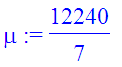
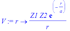
First we define some relevant parameters: we choose Bohr units, in which the electron mass equals unity, and we consider proton-atom scattering for Z2=10 (neon atoms). The Bohr potential parameter was determined from experimental scattering data for neon atoms to be a=0.52 a.u. (S. Hagmann et al. Phys. Rev. A25, p.1918ff.). A neon atom has a mass of about 20 proton masses.

>	M1:=1836: M2:=20*1836: mu:=M1*M2/(M1+M2);

>	Z1:=1: Z2:=10: a:=0.52;

>	V:=r->Z1*Z2*exp(-r/a)/r;

The procedure follows expressions as given in H. Goldstein (3rd edition), chapter 3.

First we define a procedure which computes the distance of closest approach for given initial velocity and impact parameter. It is based on the perihelion condition when the potential energy reaches its maximum along the trajectory for repulsive scattering. For given impact velocity at infinity ( v0 ) and impact parameter b  one defines the total relative scattering energy E  at infinity (zero potential), and the angular momentum magnitude L . The distance of closest approach minR  results as a solution to the energy conservation statement, which is a nonlinear equation.

>	minR:=proc(v0,b) local E,L,peri; global mu,a,Z1,Z2;

>	E:=mu*v0^2/2;

>	L:=mu*v0*b;

>	peri:=E-L^2/(2*mu*r_min^2) - V(r_min);

>	fsolve(peri,r_min=0..infinity) end:

We pick the impact velocity at infinity in Bohr units. v=1  would be intermediate value corresponding to a proton speed comparable to the classical orbit speed of a hydrogen 1s-state electron.

We would like to explore fast and slow collisions ('less' and 'more' interaction).

>

v0:=0.5;

>	r_clap:=minR(v0,2);

The distance of closest approach is slightly larger than the impact parameter.

The scattering angle is given now by eq. (3.96) in Goldstein (3rd ed). We need an integral from the distance of closest approach to infinity.

It appears as if Maple can calculate the integral numerically. It won't calculate the anti-derivative for the Bohr potential.

We reduce the precision to which the integral is computed somewhat with respect to Digits .

>	theta:=proc(v0,b) local E; global mu; E:=mu*v0^2/2;

>	evalf(Pi)-2*evalf(Int(b/(r*sqrt(r^2*(1-V(r)/E)-b^2)),r=minR(v0,b)..infinity),Digits-1); end:

>	theta(v0,0.1);

For a small impact parameter and small impact velocity a large scattering angle is found.

We now set up a loop over impact parameter. We wish to explore small and large impact parameters, because we are interested in a comparison with the unscreened Rutherford scattering case.

For small impact parameters (large deflection angles) we expect our results to agree for both potentials, as the main deflection occurs at the closest approach. For large b  values the screened case leads to tiny deflection angles which become insignificant as b  goes to infinity. In the pure Coulomb potential there is always a deflection, even as b  becomes infinite, which represents a pathology (borderline case).

>	db:=0.01; N:=200:

>	PP:=[seq([db*i,theta(v0,db*i)],i=1..N)]:

>

PP[200];

>	P1:=loglogplot(PP,style=point,color=red):

>	P2:=loglogplot(2*arccot(b*mu*v0^2/(Z1*Z2)),b=db..N*db,color=blue):

>	display(P1,P2,labels=["b","theta"],axes=boxed);

Here we see how the numerical evaluation of the integral agrees with the Rutherford result for small impact parameters. The plot for P2  is coded after eq. (3.101) in Goldstein.

It is interesting to observe that the truncation of the integral in the calculation of theta to a finite upper limit (instead of infinity) can lead to serious errors at intermediate and larger impact parameters. It means that it is essential in a numerical evaluation of the integral to map the entire integration range even for a short-range scattering potential. This is somewhat unexpected, particularly if one has investigated the theta-b  relationship using numerical solutions to the differential equation for which a rather finite integration range suffices usually.

Exercise 1:

Explore the relationship between impact parameter and scattering angle for different impact velocities while keeping all other parameters fixed. Does the b-value where the screened and unscreened results merge change with impact velocity?

Now we want to demonstrate the behaviour of the differential cross section at small angles. Does the screening of the potential prevent the cross section from blowing up at small angles?

>

PP[1];

We calculate the differential cross section using Goldstein eq. (3.93), and take the inverse of dtheta/db  to calculate db/dtheta . We calculate dsigma/dOmega  using a central finite-difference formula on the equispaced grid of b -values:

>	for i from 2 to N-1 do: dsdO[i]:=db*i/abs((PP[i+1][2]-PP[i-1][2])/(2*db))/sin(PP[i][2]); od:

In order to graph it properly as a function of the polar scattering angle we use the b -range as a parameter:

>	PPc:=[seq([PP[i][2],dsdO[i]],i=2..N-1)]:

>	P3:=loglogplot(PPc,style=point,color=red):

>	P4:=loglogplot(1/4*(Z1*Z2/(mu*v0^2))^2*csc(theta/2)^4,theta=PP[1][2]..PP[N-50][2],color=blue):

>	display(P4,P3,labels=["theta","ds/dO"],axes=boxed,title="Bohr potential(red), Coulomb potential (blue) differential cross section: dsigma/dOmega");

For the range of theta-values shown the Rutherford cross section follows a simple 1/theta^4  behaviour, as we are in the sin(theta)=theta  regime. The Bohr cross section does not blow up as badly at small angles, yet it also seems to continue to rise. To figure out what is really going on there, we need to consider much larger b -values, i.e., much smaller polar scattering angles.

We repeat the loop for the calculation with the Bohr potential:

>	db:=0.04; N:=200:

>	PP:=[seq([db*i,theta(v0,db*i)],i=1..N)]:

>	loglogplot(PP,style=point,color=red,labels=["b","theta"],axes=boxed,title="Bohr potential: theta(b)");

There appears to be a problem with noise at the larger- b  end, we should probably increase Digits . However, when we try that the calculation of the scattering angle gets stuck, because evalf(Int)  fails to return a value (the integrator can't reach the desired accuracy).

In the graph below we show dsigma/dtheta in order to address the integrability question:

>	for i from 2 to N-1 do: dsdO[i]:=db*i/abs((PP[i+1][2]-PP[i-1][2])/(2*db))/sin(PP[i][2]); od:

>	PPc:=[seq([PP[i][2],6.283*dsdO[i]*sin(PP[i][2])],i=2..N-1)]:

>	loglogplot(PPc,style=point,color=red,labels=["theta","ds/dtheta"],axes=boxed,title="Bohr potential differential cross section");

We should be aware of the fact that the cross section can't be calculated by inverting the derivative of theta'(b) when the deflection angle is so small that the absolute error in the integral exceeds the actual value. The data below demonstrate the failure of the procedure:

>	seq(dsdO[i],i=N-50..N-1);

Apparently the results for dsigma/dtheta  turn around at the smallest theta-values shown, which indicates the differential cross section is integrable.

In general, we have a hard time to verify in finite-precision arithmetic that the cross section is bounded. For some choices of scattering parameters the calculation fails before a maximum in the differential cross section is reached.

Exercise 2:

Verify the large-scattering angle regime: how well does the numerical Bohr calculation agree with the analytical Rutherford result for dsigma/dOmega ?

Mini-projects:

Explore some other repulsive central potential that has a finite range. Investigate the b-theta  relationship and the differential scattering cross section.

Investigate potentials with a power-law fall-off that decay faster than the Coulomb potential and explore the forward differential cross section.

Investigate attractive finite-range scattering potentials V(r) .

>