MomentInertia.html

MomentInertia.html MomentInertia.mws

Moment of Inertia Tensor

In this worksheet we calculate the moment of inertia matrix in a given coordinate system and show that a coordinate system can be found in which the inertia tensor is represented by a diagonal matrix.

This worksheet requires maple8 to work properly (integral I2 below won't evaluate in earlier versions, and even in maple8 it integrates with a wrong sign). For a workaround that involves some extras: consult MomentInertia7.mws in the same folder.

> restart; with(LinearAlgebra):

> with(plots): with(plottools):

Warning, the name changecoords has been redefined

Warning, the name arrow has been redefined

We start with an example for which the calculation of the integrals is relatively straightforward. We assume a homogeneous material for which the mass density is constant, and given as the ratio of total mass divided by the total volume.

> rho:=M/V;

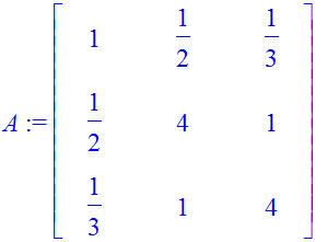
To practice our computational skills we work on an ellipsoid which is described by a quadratic form. This will be a cigar-shaped body, which has an ellipse as cross section.

> A:=Matrix([[1,1/2,1/3],[1/2,4,1],[1/3,1,4]]);

> A-Transpose(A);

The above null-result shows that A was chosen to be real and symmetric.

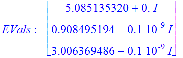
> EVals:=evalf(Eigenvalues(A));

The numerical noise in the eigenvalues (non-zero imaginary parts) comes from the evalf calculation to 10 digits (verify this by repeating the calculation with Digits set higher than the default value of 10).

The matrix has positive eigenvalues which are related to the semimajor axes of the ellipsoid. If one (or two) of them were negative our quadratic surface would be made up of hyperboloidal sheets.

We anticipate a result to be derived below: in a principal-axis frame, the quadratic form will be given as:

QF = EVals[1]*x^2 + EVals[2]*y^2 + EVals[3]*z^2

We can set QF =1 (to chose a scale), and recognize that the eigenvalues are equal to EV[i] = 1/a_i^2, where a_i are the semi-major axes.

Therefore the volume of the ellipsoid is calculated as:

> V0:=evalf(4/3*Pi*mul(sqrt(1/EVals[i]),i=1..3));

> seq(Re(sqrt(1/EVals[i])),i=1..3);

Now we calculate the quadratic form.

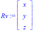
> Rv:=Vector([x,y,z]);

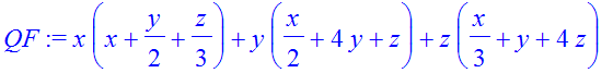
> QF:=Transpose(Rv) . A . Rv;

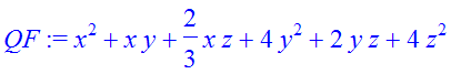
> QF:=simplify(QF);

> surf:=solve(QF-1,z);

> plot3d(surf[1],x=-1.1..1.1,y=-1.1..1.1,axes=boxed,grid=[30,30],style=patchcontour,shading=zhue,scaling=constrained);

This doesn't look so great, so it is better to use an implict plot.

> implicitplot3d(QF-1,x=-1.1..1.1,y=-1.1..1.1,z=-1.1..1.1,axes=boxed,numpoints=2000,scaling=constrained,style=patchcontour,shading=zhue);

> EVecs:=evalf( Eigenvectors(A) );

We are interested in a graph of the three eigenvectors. They are stored in the columns of the matrix (2nd entry in Evecs ). We want to show that they are orthogonal, and how they are related to the shape of the quadratic surface.

> E1v:=convert(SubMatrix(EVecs[2],1..3,1..1),Vector);

> E1v:=Normalize(map(Re,E1v),Euclidean);

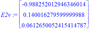
> E2v:=Normalize(map(Re,convert(SubMatrix(EVecs[2],1..3,2..2),Vector)),Euclidean);

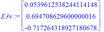
> E3v:=Normalize(map(Re,convert(SubMatrix(EVecs[2],1..3,3..3),Vector)),Euclidean);

> E1 := plottools[arrow]([0, 0, 0], E1v, .2, .4, .1, color=red):

> E2 := plottools[arrow]([0, 0, 0], E2v, .2, .4, .1, color=blue):

> E3 := plottools[arrow]([0, 0, 0], E3v, .2, .4, .1, color=green):

> QFp:=implicitplot3d(QF-1,x=-1.1..1.1,y=-1.1..1.1,z=-1.1..1.1,axes=boxed,numpoints=2000,scaling=constrained,style=wireframe,color=gold):

> display(E1,E2,E3,QFp,axes=boxed);

> E1v . E2v;

> E1v . E1v;

> E1v . E3v;

> E2v . E3v;

Rotate the above graph to obtain a clear understanding of the geometry.

Exercise 1:

Change the matrix in the above quadratic form and repeat the steps.

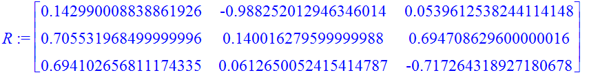
We proceed with constructing an orthogonal matrix out of the normalized eigenvectors. We then transform the matrix to demonstrate that it is diagonalized by this transformation.

> R:=Matrix([E1v,E2v,E3v]);

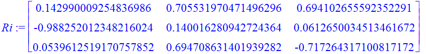
> Ri:=MatrixInverse(R);

Our transformation matrix made up of the eigenvectors as columns is orthogonal, i.e., the inverse is given by the transpose.

We now calculate the transformation of matrix A by the matrix R, the correct form is Ri . A . R (the other way around doesn't work as shown below!)

> Ri . A . R;

The transformed matrix has the eigenvalues on the diagonal, and zeroes (approximately) for all non-diagonal entries.

> R . A . Ri;

Exercise 2:

Calculate the quadratic form using the diagonalized matrix. Truncate the near-zero entries to zero, i.e., make up a diagonal matrix from the eigenvalues and observe the equation for the quadratic form (absence of cross terms).

Carry out the transformation to the principal axes frame (as done above) for some other matrix A with three positive eigenvalues.

Volume calculation.

Can we calculate the volume V in Cartesian coordinates? We choose the quadratic form with scale factor 1.

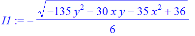
Let us do the repeated integrals one at a time. First the z integration:

> fz:=solve(QF-1,z);

> I1:=int(1,z=fz[1]..fz[2]);

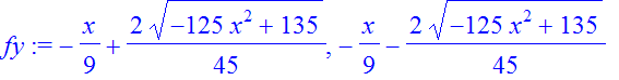
> fy:=solve(I1,y);

> plot([fy[1],fy[2]],x=-1.1..1.1,color=[red,blue],numpoints=800,scaling=constrained);

Following the z-integration we need to integrate I1 over an area bounded by the curves fy[1] and fy[2] .

We will integrate over y between the lower (blue) and upper (red) bounding curves. Then we will integrate over x between fixed limits. What are these limits?

They are the points where the derivative y(x) goes to infinity.

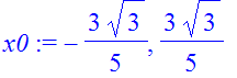
> x0:=solve(1/diff(fy[1],x),x);

The direct attempt of definite integration is not successful:

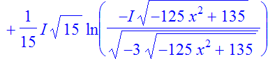
> I2:=int(I1,y=fy[1]..fy[2]);

> I3idf:=int(expand(I2),x);

We should be able to do this integral at least numerically. We need to know the range of x:

> evalf(x0);

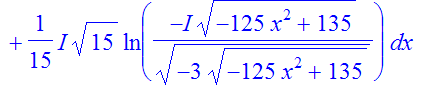
> plot(I2,x=x0[1]..x0[2]);

Somehow maple8 made a mistake: it chose a branch cut for the ln function which turned our results upside down. We need to integrate this function, and do it numerically and correct the sign:

> V:=evalf(Int(-I2,x=x0[1]..x0[2]));

> V0:=evalf(4/3*Pi*mul(sqrt(1/Eigenvalues(A)[i]),i=1..3),15);

The volume integration worked! We carried out two of the three integrations analytically, and then the third one numerically.

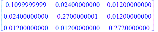
Now we calculate the moments of inertia matrix .

>

> M:=1; rho;

> MI:=Matrix(3,3):

> for i from 1 to 3 do: for j from 1 to i do:

> if i=1 and j=1 then w:=Rv[2]^2+Rv[3]^2; elif i=2 and j=2 then w:=Rv[1]^2+Rv[3]^2; elif i=3 and j=3 then w:=Rv[1]^2+Rv[2]^2; else w:=-Rv[i]*Rv[j]; fi:

> I1:=int(w*rho,z=fz[1]..fz[2]);

> I2idf:=unapply(int(I1,y),y);

> I2:=expand(I2idf(fy[2])-I2idf(fy[1]));

> I2:=simplify(I2);

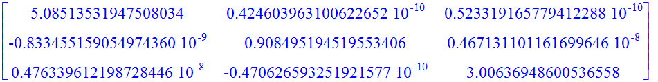
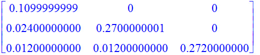
> MI[i,j]:=evalf(Int(I2,x=x0[1]..x0[2]));

> od: od:

> print(MI);

Now fill the complete matrix by symmetry:

> for i from 1 to 3 do: for j from i to 3 do: MI[i,j]:=MI[j,i]: od: od:

> print(MI);

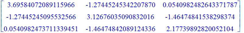
> Eigenvalues(MI);

These are the principal moments of inertia.

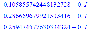
> EVecsMI:=Eigenvectors(MI);

We are interested in a graph of the three eigenvectors.

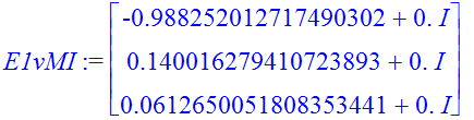
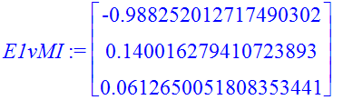
> E1vMI:=convert(SubMatrix(EVecsMI[2],1..3,1..1),Vector);

> E1vMI:=Normalize(map(Re,E1vMI),Euclidean);

> E2vMI:=Normalize(map(Re,convert(SubMatrix(EVecsMI[2],1..3,2..2),Vector)),Euclidean);

> E3vMI:=Normalize(map(Re,convert(SubMatrix(EVecsMI[2],1..3,3..3),Vector)),Euclidean);

> RMI:=Matrix([E1vMI,E2vMI,E3vMI]);

> R;

> E1MI := plottools[arrow]([0, 0, 0], E1vMI, .2, .4, .1, color=red):

> E2MI := plottools[arrow]([0, 0, 0], E2vMI, .2, .4, .1, color=blue):

> E3MI := plottools[arrow]([0, 0, 0], E3vMI, .2, .4, .1, color=green):

The eigenvectors of the MI matrix provide those axes about which rotation of the body without deviation moments is possible.

Note that as in the 'spinning textbook' problem the motion about the axes with extreme eigenvalues will be truly stable, while free rotation about the axis associated with the intermediate eigenvalue results in a wobble (instability in Euler's equation).

The remarkable thing about rotational mechanics is that for any shape (e.g., a potato) three axes can be found about which pure rotation is possible without deviation moments. The ellipsoid is as close a mathematical form that we can handle that describes such a potato. The diagram below illustrates that the stable rotation axes do coincide with the axes that are perpendicular to the elliptic cross sections.

> display(E1MI,E2MI,E3MI,QFp,axes=boxed);

The eigenvectors of the moment of inertia matrix look the same as the eigenvectors that diagonalize the quadratic form. Here is an example of two matrices that share a set of eigenvectors, but have different eigenvalues.

We observe that vectors can be found which are at the same time eigenvectors of matrix A (which defines the geometric shape), and of the moment of inertia matrix MI. These two matrices are distinct and have distinct eigenvalues. According to a theorem in linear algebra a common set of eigenvectors can be found for two matrices if they commute with each other, i.e., wenn the product A.B is the same as B.A :

Let us explore the properties:

First, the orthogonality of the eigenvectors of the MI matrix:

> E1vMI . E2vMI;

> E1vMI .E1vMI;

Of course, the eigenvectors of the MI matrix are perpendicular. Try the others by editing the above lines.

The following three lines indicate which eigenvectors of the MI matrix correspond to the principal axes of the ellipsoid:

> E1v . E1vMI;

> E2v . E1vMI;

> E3v . E1vMI;

The first eigenvector of the MI matrix corresponds to the second eigenvector of the quadratic form.

> E1v . E2vMI;

> E2v . E2vMI;

> E3v . E2vMI;

The second eigenvector of the MI matrix corresponds to the first eigenvector of the quadratic form.

> E1v . E3vMI;

> E2v . E3vMI;

> E3v . E3vMI;

Here we have a sign change. Eigenvectors are defined up to a multiplicative constant. We display all vectors and teh QF:

> display(E1,E2,E3,E1MI,E2MI,E3MI,QFp,axes=boxed);

Let us calculate the commutator of the two matrices, namely the one defining the QF and the MI matrix:

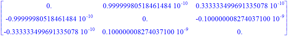
> A . MI - MI . A;

Indeed, the product A . MI is within numerical accuracy the same as the product MI . A !

Exercise 3:

Explore the relationship between the principal axes of the quadratic form, and the principal axes of the moment of inertia matrix. Try matrices A for which the form is close to a nearly circular cross section, i.e., find matrices A such that two of the eigenvalues are very close.

What happens to the eigenvectors when two eigenvalues are very close? What shape do you get when three eigenvalues are close?

>