 �
�
� Wigner distribution �
��
�� The Wigner function is the basic quantity to describe ensembles in a phase-space formulation of quantum mechanics. It is defined as a paricular Fourier transform of the density matrix. �
�� f(q,p) = int(exp(-I*p*s)*psi(q+s/2)*psi^*(q-s/2),s=-infinity..infinity) �
�� (the integral corresponds to an inverse Fourier transform) �
��
�� Let us start with the simplest examples, such as harmonic oscillator eigenstates: �
��
| > | �restart; with(inttrans): � |
�
| > | �fx:=x*exp(-x^2/2); #chose the unnormalized state here � |
�
 �
�
�
| > | �No:=1/sqrt(int((fx)^2,x=-infinity..infinity)); � |
�
 �
�
�
| > | �psi:=unapply(No*fx,x); � |
�
 �
�
�
| > | �int(psi(x)^2,x=-infinity..infinity); � |
�
![]() �
�
�
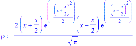
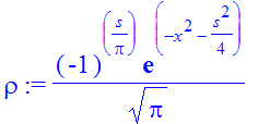
| > | �rho:=psi(x+s/2)*psi(x-s/2); � |
�
 �
�
�
| > | �fW:=invfourier(rho,s,p); � |
�
 �
�
�
| > | �Rp:=int(fW,x=-infinity..infinity); � |
�
 �
�
�
| > | �Rx:=int(fW,p=-infinity..infinity); � |
�
 �
�
�
| > | �plot(Rx,x=-3..3); � |
�
![[Maple Plot]](images/Wigner9.gif) �
�
�
| > | �int(Rp,p=-infinity..infinity); � |
�
![]() �
�
�
| > | �int(Rx,x=-infinity..infinity); � |
�
![]() �
�
�
| > | �plot3d(fW,x=-3..3,p=-3..3,axes=boxed,shading=zhue); � |
�
![[Maple Plot]](images/Wigner12.gif) �
�
� Nothing particularly exciting happens here for the ground state. For the first excited state we have something non-classical: the Wigner function is not positive definite! �
��
�� Exercise 1: �
�� Choose different excited states of the harmonic oscillator and calculate the Wigner function. How is the number of nodes in the wavefunction related to the structure in phase space? �
��
�� What do we obtain for a wavepacket? �
��
�� We choose a Gaussian wavepacket centered at the origin with an average momentum of � p0 � . We pick a simple width (which controls the width of the momentum distribution for all times). We compute the answer at time zero. �
��
| > | �p0:=1; � |
�
![]() �
�
�
| > | �fx:=exp(-(x)^2/2)*exp(I*p0*x); #chose the unnormalized state here � |
�
 �
�
�
| > | �#fx:=1/(1+x^2)*exp(I*p0*x); # the Lorentzian wavepacket doesn't work. � |
�
| > | �No:=1/sqrt(int(abs(fx)^2,x=-infinity..infinity)); � |
�
 �
�
�
| > | �psi:=unapply(No*fx,x); � |
�
 �
�
�
| > | �int(abs(psi(x))^2,x=-infinity..infinity); � |
�
![]() �
�
�
| > | �assume(x,real,s,real); � |
�
| > | �rho:=simplify(expand(psi(x+s/2)*conjugate(psi(x-s/2)))); � |
�
 �
�
�
| > | �fW:=invfourier(rho,s,p); � |
�
 �
�
�
| > | �Rp:=int(fW,x=-infinity..infinity); � |
�
 �
�
�
| > | �Rx:=int(fW,p=-infinity..infinity); � |
�
 �
�
�
| > | �plot([Re(Rp),Im(Rp)],p=-3..3,color=[red,blue]); � |
�
![[Maple Plot]](images/Wigner22.gif) �
�
� Something went wrong. The Wigner function should be real-valued. �
��
| > | �int(Rx,x=-infinity..infinity); � |
�
![]() �
�
�
| > | �fW:=simplify(expand(int(exp(-I*p*s)*rho,s=-infinity..infinity))); � |
�
![]() �
�
�
| > | �subs(p=1,x=1,%); � |
�
![]() �
�
�
| > | �plot3d(fW,x=-3..3,p=-3..3,axes=boxed,shading=zhue); � |
�
![[Maple Plot]](images/Wigner26.gif) �
�
� The Wigner function for a Gaussian wavepacket state is quite straightforward, and is easily interpreted. �
��
�� Exercise 2: �
�� Displace the Gaussian wavepacket and re-compute the Wigner function. �
��
�� Exercise 3: �
�� Broaden the Gaussian wavepacket in coordinate space and re-compute the Wigner function. Make your observation about the momentum distribution. �
��
�� We explore now the time-dependent Gaussian wavepacket. The width parameter � a � determines the spatial extent and momentum spread about the average. �
��
| > | �a:=1; p0:='p0'; � |
�
![]() �
�
�
![]() �
�
�
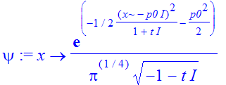
| > | �psi := unapply(sqrt(a)*1/Pi^(1/4)*exp(-1/2*(x-I*a^2*p0)^2/(a^2+t*I)-1/2*a^2*p0^2)/(sqrt(-a^2-I*t)),x); � |
�
 �
�
�
| > | �assume(t>0); � |
�
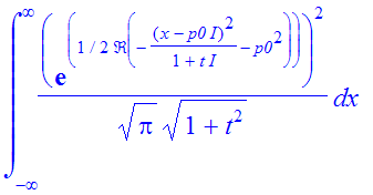
| > | �int(abs(psi(x))^2,x=-infinity..infinity); � |
�
 �
�
�
| > | �int(evalc(simplify(abs(psi(x))^2)),x=-infinity..infinity); � |
�
![]() �
�
�
| > | �rho:=simplify(expand(psi(x+s/2)*conjugate(psi(x-s/2)))); � |
�
![]() �
�
 �
�
�
| > | �fW:=simplify(expand(int(exp(-I*p*s)*rho,s=-infinity..infinity))); � |
�
 �
�
�
| > | �fW:=evalc(fW); � |
�
 �
�
�
| > | �p0:=1; � |
�
![]() �
�
�
| > | �fW1:=subs(t=1,fW); � |
�
![]() �
�
�
| > | �fW2:=subs(t=2,fW); � |
�
![]() �
�
�
| > | �fW3:=subs(t=3,fW); � |
�
![]() �
�
�
| > | �Rx1:=int(fW1,p=-infinity..infinity); � |
�
![]() �
�
�
| > | �Rx2:=int(fW2,p=-infinity..infinity); � |
�
 �
�
�
| > | �Rx3:=int(fW3,p=-infinity..infinity); � |
�
 �
�
�
| > | �plot([Rx1,Rx2,Rx3],x=-5..10,color=[red,blue,green]); � |
�
![[Maple Plot]](images/Wigner43.gif) �
�
�
| > | �Rp1:=int(fW1,x=-infinity..infinity); � |
�
![]() �
�
�
| > | �Rp2:=int(fW2,x=-infinity..infinity); � |
�
![]() �
�
�
| > | �Rp3:=int(fW3,x=-infinity..infinity); � |
�
![]() �
�
� The momentum distribution remains constant! This is required, since the wavepacket undergoes free dispersion. �
��
| > | �plots[animate3d](fW,x=-5..15,p=-4..4,t=0..4,axes=boxed,grid=[50,50],shading=zhue,style=patchcontour,frames=20); � |
�
![[Maple Plot]](images/Wigner47.gif) �
�
� The apparent ripples at later times are an artefact of the graphing algorithm. �
��
�� Exercise 4: �
�� Observe what happens when the spatial width parameter � a � is increased or decreased. �
��
| > | �
�
| > | �