---

Soukoreff, R. W., & MacKenzie, I. S. (2004). Towards a standard for pointing device evaluation: Perspectives on 27 years of Fitts' law research in HCI. International Journal of Human-Computer Studies, 61, 751-789. [software]

---

Towards a Standard for Pointing Device Evaluation: Perspectives on 27 Years of Fitts' Law Research in HCI

R. William Soukoreff^* and I. Scott MacKenzie

Department of Computer Science and Engineering
York University
Toronto, Ontario, Canada

Abstract
This paper makes seven recommendations to HCI researchers wishing to construct Fitts' law models for either movement time prediction, or for the comparison of conditions in an experiment. These seven recommendations support (and in some cases supplement) the methods described in the recent ISO 9241-9 standard on the evaluation of pointing devices. In addition to improving the robustness of Fitts' law models, these recommendations (if widely employed) will improve the comparability and consistency of forthcoming publications. Arguments to support these recommendations are presented, as are concise reviews of 24 published Fitts' law models of the mouse, and 9 studies that used the new ISO standard.

Keywords:
Fitts' law, human performance modelling, motor control, pointing device evaluation, bandwidth, index of performance, ISO 9241-9.

1.0 Introduction

Fitts' law (1954)¹ describes the relationship between movement time, distance, and accuracy for people engaged in rapid aimed movements. It has been verified over a wide range of conditions.² Of interest to HCI researchers is that the law applies to pointing and dragging using a mouse, trackball, stylus, joystick, and touchscreen. Fitts' law has been applied by HCI researchers in primarily two ways, as a predictive model, and as a means to derive the dependent measure throughput (defined later in this paper).

As a predictive model, Fitts' law directly applies to many problems in HCI. For example, one can use Fitts' law to predict the time for the user of a graphical interface to move the mouse tracker to a button and click on it. This concept can be extended: the time required to type a word using a stylus on a soft-keyboard can be predicted by summing the Fitts' movement times of a series of letter-to-letter stylus movements over the keyboard (Soukoreff & MacKenzie, 1995). Using the keystroke-level model one can predict the time to accomplish an interaction that is more complicated than simple clicking, such as editing a document. This is accomplished by breaking complex interactions into an appropriate series of sub-actions (where a Fitts' law movement is one of the sub-actions) and summing the time for each (Card, Moran, & Newell, 1980). This predictive aspect of Fitts' law can be directly applied to interface design, for example, by keeping frequently-used targets close to the tracker (e.g., with a pop-up menu), or by increasing the target-icon size for longer movements (Newell & Card, 1985, page 223).

The second way Fitts' law is used in HCI is as part of the comparison and evaluation of novel pointing devices. Essentially, this application turns Fitts' law inside-out: instead of using it to predict movement times, researchers measure several movement times and then determine how the different conditions affect the coefficients within the Fitts' law relation. Thus, Fitts' law has demonstrated its utility to compress several movement time measurements into the single statistic, throughput, that combines both speed and accuracy.³ The value of this measure has been recognised by academic and industry researchers alike, as it has been codified in a recent ISO standard describing the evaluation of pointing devices (ISO, 2002). Although only two years since final adoption, this standard is already used by several research groups (Douglas, Kirkpatrick, & MacKenzie, 1999; Isokoski & Raisamo, 2002; Keates, Hwang, Langdon, Clarkson, & Robinson, 2002; MacKenzie & Jusoh, 2001; MacKenzie et al., 2001; MacKenzie & Oniszczak, 1998; Oh & Stuerzlinger, 2002; Poupyrev, Okabe, & Maruyama, 2004; Silfverberg, MacKenzie, & Kauppinen, 2001).

The purpose of this paper is to make recommendations regarding how to use Fitts' law in the two application areas described above. Between 1954 (the year Fitts' law was first described in the literature) and 1978 (the first time Fitts' law was used in an HCI paper, Card, English, & Burr, 1978), Fitts' law underwent refinements in three areas: in its mathematical formulation, in the accommodation of the distribution of movement end-points, and in the means to calculate pointing device throughput. (Each of these points is elaborated later in this paper.) However, these refinements are not universally accepted and as a result we are faced with a seemingly endless multiplicity of variations of the law, rendering much of the literature inconsistent and incomparable (see section 5.5 - Summary, in MacKenzie, 1992a). As researchers, we must strive toward a standard, so that our results comprise a consistent body of research, instead of contributing to the problem by generating even more incongruent papers. Some progress toward a standard is evident. As mentioned, in 2002 the ISO9241-9 standard was published (ISO, 2002). The next step is for researchers to adopt either this standard or methodological approaches that are compatible with this standard, for the good of the collective body of our research.

Given the free-reign with Fitts' law that HCI researchers have exercised for some time, some may have lingering concerns that a standard could stifle research. This should not be the case. The intent is to generate a commonality so that publications from different research groups contribute in a constructive way to a coherent body of work. Further, we must allow the standard to be updated to reflect the improved understanding and novel applications of Fitts' law that will inevitably come with time.

In this paper we will make seven recommendations to researchers using Fitts' law. We feel the reader will benefit from a presentation of our seven recommendations early in this paper, and so our position is summarised in the following section. After the summary, justifications of the recommendations are provided. We conclude with a brief look at the state of the published literature.

2.0 Applying Fitts' Law in HCI

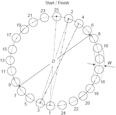
When building a Fitts' law model, one presents subjects with specific movement tasks to perform over a range of amplitudes and with a set of target widths. The physical configuration is termed the Fitts paradigm, and appears in Figure 1. The Fitts paradigm as illustrated is somewhat antiquated because angle of movement confounds pointing device performance. For this reason the ISO standard recommends a circular arrangement of targets, see Figure 2.

Figure 1 - The Fitts' paradigm (one-dimensional, horizontal). This figure depicts the Fitts paradigm — the physical layout of targets used when acquiring data from which to build a Fitts' law model. Two schemes may be used. a) The discrete task has subjects begin with the pointing device tracker at the start position and move to within the target. (This task is repeated.) b) The serial task has subjects tap back-and-forth between two targets.

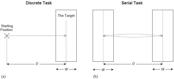
Figure 2 - Multi-directional tapping task. This illustrates the multi-directional tapping task described in the ISO9241-9 standard (2002). This paradigm has the advantage of controlling for the effect of direction. Circular or square targets may be used. The path the subject follows begins and ends in the top target. The arrows indicate the path subjects follow using the pointing device, to alternating targets clockwise around the circle. Software to capture subjects' movement times must graphically indicate which target the subject should proceed to next.

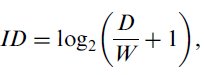
(I)⁴ When designing an experiment, researchers should use the Shannon formulation⁵ of the index of difficulty (ID),

(1)

where the units of ID are bits.⁶

(II) The variety of movement distances (D) and target widths (W) should be chosen so that subjects face a large and representative range of ID values. A range of ID values from 2 to 8 bits should suffice for most situations. A variety of index of difficulty conditions should be used regardless of which experiment paradigm (Figures 1 and 2 above) is being used.⁷

Each condition must be presented to each subject many (perhaps, 15 to 25) times, so that the central tendency of each subject's performance for each condition can be ascertained.

The experimenter should also collect movement time (MT) data. Movement time refers to the time subjects spend moving the pointing device, and specifically should not include homing time, dwell time, or reaction time if a discrete task is used.

(III) A measure of the scatter of subjects' movement end-points must be gathered, either by determining the error rate or by recording the physical end-points of each movement task. Ideally both error rates and end-points should be measured and reported.

The suggestion that experimenters record movement end-points and error rates implies that no filtering of the data (barring the removal of outliers) is performed. Specifically, "peak error-free performance" is an uninformative measure, as speed measurements in the absence of accuracy are meaningless. However, obvious outliers⁸ may be removed from the data.

(IV) The end-point scatter data should be used to perform the adjustment for accuracy for each subject, for each condition. There are two ways to accomplish this; if end-point scatter data has been observed, then the standard deviation (σ) of the end-point positions should be calculated,⁹ and the effective target width (We) is then defined as

(2)

Alternately, the error rate may be used to approximate the adjustment for accuracy, if the standard deviation of the end-point data is unavailable,

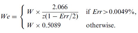
(3)

where Err is the error rate corresponding to this specific condition, and z(x) represents the inverse of the standard normal cumulative distribution, or, the z-score that corresponds to the point where the area under the normal curve is x%. For example, z(96%) = 1.75069 (in other words, P[z ≥ 1.75069] = 96%).¹⁰

If the movement end-point data are available, the movement distance parameter D can also be adjusted for accuracy. The effective distance, De, is calculated as the mean movement distance from the start-of-movement position to the end position.

The adjusted width parameter (and adjusted distance — if available) are used to define the effective index of difficulty,

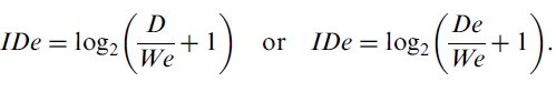
(4)

The interpretation of the adjustment for accuracy follows. The ID values calculated via Equation 1 above represent the movement tasks that the experimenter wants subjects to attempt to perform. However, the subjects will not actually perform at these index of difficulty values for two reasons. (i) The spread of movement end-points will not perfectly align with the target widths specified and hence the error rates will not be consistent across the various ID values. (ii) Subjects tend to 'cheat' on easier ID conditions by not moving fast enough,¹¹ and by not covering the whole distance (they click just inside the edge of near, wide targets). The disparity between subjects' performance and the ID values presented by the experimenter is greatest at the extremes — the highest and lowest ID values used. The adjustment for accuracy corrects the ID values so that they match the movements that subjects actually performed.

A large discrepancy between ID and IDe should be acknowledged and noted. The difference between ID and IDe is a natural consequence of motivated subjects' desire to perform well. However, a large discrepancy may indicate that the movement tasks were ill-suited to the pointing device under investigation.

Another point for further clarification concerns the treatment of separate conditions with identical ID values. Consider the conditions used in Fitts' seminal (1954) publication, presented in Table 1. Sixteen conditions gave rise to seven distinct ID values. This does not mean that there are only seven distinct conditions! The adjustment for accuracy has the systematic effect of slightly increasing low ID values, and decreasing high ID values. So after the adjustment for accuracy has been performed, the ID values for each condition typically spread to distinct values. Just to be clear, the parameters used for the adjustment for accuracy (i.e., the end-point distribution or error rates) for each condition should be treated distinctly, even if some of the conditions do have identical ID values.

Table 1
ID Values From Fitts' (1954) Paper

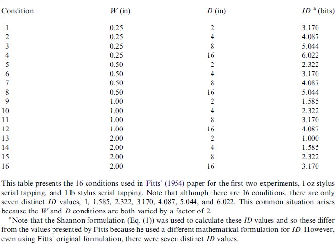
This table presents the sixteen conditions used in Fitts' (1954) paper for the first two experiments, 1-oz stylus serial tapping, and 1-lb stylus serial tapping. Note that although there are sixteen conditions, there are only seven distinct ID values, 1, 1.585, 2.322, 3.170, 4.087, 5.044, and 6.022. This common situation arises because the W and D conditions are both varied by a factor of 2.

Yet another point of clarification concerns the pooling of subjects' data. The adjustment for accuracy must be performed for each condition faced by each subject, because it makes use of within-subject variability. Thus the movement end-points or error rates used to perform the adjustment for accuracy cannot be pooled together; correct application of the adjustment for accuracy requires separate measurements for each subject, for each condition.

By the end of this step in the analysis, if there were y subjects and x conditions, the experimenter should have n = y × x pairs of movement time and effective index of difficulty data, (IDe_ij, MT_ij) where 1 ≤ i ≤ y and 1 ≤ j ≤ x.

(V) Least-squares linear regression is used to find the intercept (a) and slope (b) parameters of the Fitts' law equation,¹²

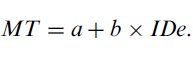
(5)

Linear regression serves as a test to measure the goodness of fit (is there a linear relationship between movement time and the index of difficulty?), and the reasonableness of the results. Due to the natural variability of human performance, the intercept (a in Equation 5) will not be exactly zero, but the absolute value of the intercept parameter of the regression model (a) must be a small value. If the intercept is positive, it should be under 400 ms, but preferably smaller still. Negative intercept values occur in the literature, and tend to be smaller in magnitude than positive intercepts, and hence probably should not exceed −200 ms. If the magnitude of the intercept is larger, then an explanation is warranted. There are legitimate reasons that such a situation may occur — but often, we fear, a large intercept indicates a problem with the experiment methodology. Were the movement times measured accurately? Did subjects move quickly and with no delays? Was homing time, dwell time, and reaction time (if applicable) accounted for so they don't artificially inflate movement time? Is there an intrinsic reason why the pointing-device under examination slows subjects, increasing reaction times or movement times? Do expert subjects (as opposed to 'normal' and novice subjects) also exhibit a large intercept? Have subjects received enough practice so that learning is not a factor.¹³ A large intercept value in the absence of an explanation indicates a problem with the methodology.

A statistical test is available to determine whether the intercept of a regression equation is significantly different from zero (Sen & Srivastava, 1990). The formulae are provided below.¹⁴ An estimate of the variance of the regression model can be calculated,

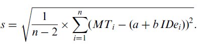
(6)

Given the mean effective index of difficulty we can calculate the standard error of the intercept, s.e.(a), with,

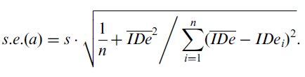
(7)

Finally, a statistic following the student's t distribution with (n − 2) degrees of freedom is obtained by dividing the absolute value of the intercept by its standard error. The probability of observing an intercept as extreme as a given that the intercept is really zero, is,¹⁵

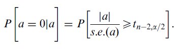
(8)

This probability indicates whether the intercept of the regression model, a, is significantly different from zero.

(VI) At this point in the analysis, we have obtained the Fitts' law regression model formulated as per Equation 5. If our intent is to make movement time predictions using the model, then movement time should be predicted using Equation 9.

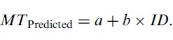
(9)

Note that the index of difficulty values used for prediction are distinct from the IDe values used for generating the model. When calculating predictions, one does not know what the distribution of movement end-points will be, and hence we cannot apply the adjustment for accuracy. Also, predictions so made carry an inherent 4% error probability (this is discussed further, below, in section 3.2).

The values of ID should be calculated using the Shannon formulation (Equation 1, above). Care must be taken that the ID values used for making predictions lie strictly within the range of IDe values that were used when constructing the model. This requirement arises because it is not valid to make predictions using a regression model outside of the range of the independent variable used to construct the model. This applies also to the intercept. The intercept should not be used to model the time required for clicking or tapping in place, as (i) the intercept is always outside the domain of the regression model,¹⁶ (ii) Fitts' law applies to rapid aimed movements — it does not apply to tapping in place where no lateral movement occurs, and (iii) Fitts' law tends to underestimate the time required for tapping in place. (This issue is discussed further in the 'justification' section that follows, see Footnote 30.)

(VII) If the purpose of this analysis is the comparison of two or more experiment conditions, then throughput (TP) is calculated first for each subject (as the mean throughput achieved by the subject over all x movement conditions), and these subject throughputs are averaged to produce the grand throughput,

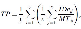
(10)

where y is the number of subjects, and x represents the number of movement conditions. The units of throughput are bits per second (or bps).

Calculated this way, TP is a complete measure encompassing both the speed and accuracy of the movement performance. Speed and accuracy are averaged over the range of IDe values used in the study, and as such, this approach combines the effects of the intercept and slope parameters of the regression model into one dependent measure that can easily be compared between conditions (and, indeed, between studies). This dependent measure may be tested for significance using an ANOVA.

Although TP provides a useful over-all measure of performance, movement times (means for each ID condition), error rates (per condition), and end-point variation (the standard deviation of end-point positions, per condition) complete the picture, and should be included in published reports.

Above we described the recommended way to construct a Fitts' law model, and seven specific recommendations were made. Next we present arguments justifying these recommendations.

3.0 Justification of the Recommendations

In the previous section of this paper we described the recommended approach to building a Fitts' law model. Seven specific recommendations were made:

I.		Use the Shannon formulation of ID (Equation 1).
II.		Use a wide and representative range of ID values (ID values ranging from 2 to 8 bits should apply to most situations).
III.		Measure the scatter of movement end-point positions , using error rates and/or end-point data.
IV.		Perform the adjustment for accuracy to convert the ID values to IDe values. Note Any large discrepancy between the ID and IDe values.
V.		Use linear regression to measure the goodness of fit (to decide whether Fitts' law indeed applies) and to verify that the intercept (a in Equation 5) is small. Investigate and explain a large intercept value.
VI.		Limit predictions made from the resulting Fitts' law linear regression model to the range of IDe values used (and specifically, the intercept should not be misconstrued as the time to make a zero-distance movement).
VII.		If devices or experiment conditions are to be compared, calculate the dependent measure throughput via the mean of means (Equation 10).

We begin our justification of these recommendations with some statements regarding the theoretical basis of Fitts' law.

3.1 The Theoretical Basis of Fitts' Law

Although Fitts' law is often used to predict movement time performance for rapid aimed movements with a good fit to empirical data, no satisfactory psychomotor theory exists that explains Fitts' law.¹⁷ But this is not a shortcoming — the accuracy, utility, and simplicity, of Fitts' law justify our continued interest in, and use of, this relation.

Fitts' 1954 paper is usually cited in the literature as the seminal Fitts' law paper, but Fitts published a little-known paper the year before (1953) in which he describes the Fitts movement paradigm (including the same apparatus used in his 1954 paper), and presents the formulation for ID that would later bare his name. This earlier paper provides interesting insight into how Fitts arrived at the relation we now call Fitts' law. Fitts wrote that "the approximate model for such a task... is the information source rather than the transmission channel... performance can be taken as a measure of [one's] capacity for performing repetitive motor tasks under varying conditions". (Fitts, 1953, page 61) Fitts viewed his relation as a means to measure the information capacity to manipulate a limb making a rapid aimed movement. Viewed as such, Fitts' law rises above the psychological, biological, and physical means the body employs to accomplish movement. The theoretical underpinnings lie in information theory, not biomechanics, and so it is to information theory that we now turn our attention. Fitts cites Shannon's theorem 17 as the basis of his law. (Fitts, 1954; Shannon & Weaver, 1949) Shannon's work provides two things useful to us in the discussions that follow, the first is his theorem 17, and the second is an observation concerning the maximum entropy of a communications channel.

Shannon's theorem 17 describes the information capacity of a continuous channel in the presence of noise, and specifically, that the channel capacity is equal to the difference between the entropy of the signal and the noise, or,

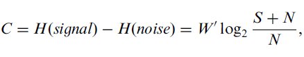
(11)

where H(•) represents the entropy of the given quantity, W′ represents the bandwidth of the communications channel,¹⁸ and S and N represent the average power of the signal and noise, respectively. (Shannon & Weaver, 1949, Part III: Mathematical Preliminaries, Section 20: Entropy of a Continuous Distribution, Claim 8)¹⁹ Comparing Equations 1 and 11 the information theoretic basis for Fitts' law is quite apparent. Fitts took the movement distance as analogous to the signal, and similarly the target width as the noise.

One might wonder what properties the signal and noise have that affect their individual entropies. Continuous data are comprised of signals²⁰ that follow a probability distribution, and it is the probability distribution that affects the information content. A question that naturally arises from this is, what continuous probability distribution yields the maximum entropy? The answer is the Normal (Gaussian) distribution.²¹ (Shannon & Weaver, 1949, Part III: Mathematical Preliminaries, Section 20: Entropy of a Continuous Distribution, Claims 5 and 6) Further, the entropy of a Normally-distributed continuous signal is a function of the standard deviation, specifically,

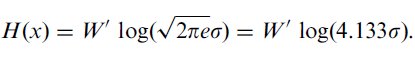
(12)

Intuitively, Equation 12 means that if the data have a wider distribution (i.e., is more variable) they embody more information than if the data are narrow.

We may now consider how Fitts' law is affected by the probability distribution of the data it is used to model.

3.2 Fitts' law and Accuracy

Crossman describes Fitts' law in a similar manner to how Shannon defined his theorem 17, "as the difference between an initial entropy... and a final one..., and hence it represents the reduction of uncertainty of the endpoint of movement achieved on a single tap." (Crossman, 1960, page 11) And since we know (from the previous section) that information content is affected by the distribution of data, we must wonder what affect statistical variations in the movement tasks have upon Fitts' law. We address this question by returning to that early paper by Fitts.

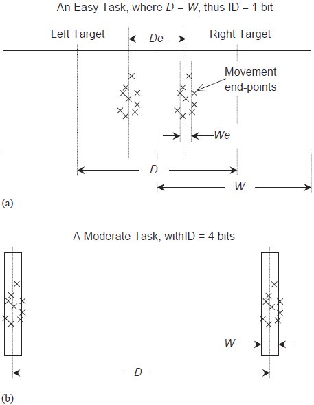
"Although the proposed unit has some resemblance to the unit of information it will be desirable to call it by another name for the present. It will be referred to hereafter as a Binary Index of Task Difficulty. It is not an exact measure of information because no account is taken of errors and no distinction is made between movements that terminate at the exact center of a target and those that terminate near the edges." (Fitts, 1953, page 64)

Fitts recognised, even at this early stage, that the distribution of movement end-points was a confounding factor. Fitts' law, like Shannon's theorem 17, depends upon the difference between two information sources. If the distribution of a subject's movement end-points is too narrow (viz., has a smaller variance) then less information is contained in the width information source (see Equation 12) and so, in total, more information is actually communicated. (The converse is true of too wide a spread of movement end-points.) In Shannon's domain, this is equivalent to reducing the noise and hence increasing the information capacity of the channel. The problem is that subjects do not perform at a consistent level of accuracy across all ID conditions.²² When presented with an easy task (see Figure 3a) subjects typically do not use the entire target width for their movements, as they do when faced with a moderately difficult task (Figure 3b). At the difficult end of the spectrum (not shown) subjects must squeeze their movement end-points together to keep them satisfactorily within the bounds of narrow, distant targets. So, we can ask subjects to attempt any task we want (by this we mean that the experimenter chooses the ID value to present), but in the end the quantity of interest is the throughput that subjects actually achieve.

Figure 3 - Subject performance under different ID conditions. This figure demonstrates the important difference between the parameters of the movement task that experimenters set for subjects, and the task that subjects actually perform. a) Consider a task at the easy extreme of the ID continuum. Because the targets are so close (in fact, they are touching) subjects are not likely to spread their end-points over the whole target. This is because subjects do not go fast enough to cause the spread of their movement end-points to make use of the entire target widths. Consequently, they are not likely to commit any errors, and the effective distance and width bear little resemblance to the task set for them. b) In a task of moderate difficulty the parameters of the task assigned and the observations are more likely to be similar.

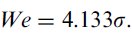
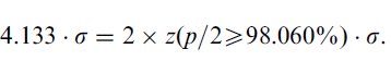
It was Crossman (1957)²³ who proposed a means to account for a subject's accuracy — a technique we now call the adjustment for accuracy. The idea is to normalise the target widths to some (physical) extent in such a way as to account for the differing spread of movement end-points that occurs during the various ID conditions. To clarify, we're not trying to make the variability of movement end-points (hence entropy) the same for each condition, rather, the goal is to define an effective target width (We) that is representative of the spread of data. Assuming the movement end-points are normally distributed²⁴ about a mean (corresponding to the centre of the effective target) with a particular standard deviation, then one can calculate the information content of the distribution of the movement end-points. This corresponds to Equation 12 which reveals that the maximum entropy is 4.133 times the standard deviation of the movement end-point positions, providing a measure of distance (width) that (i) encompasses the variability of observed data, (ii) is easy to calculate, and (iii) is consistent with the information theory that Fitts' law is based on, and analogous to. Thus we have the definition for We as given in Equation 2.

When movement end-point data are not available, an approximation of the adjustment for accuracy is found from the error rate. This approximation arises by observing that a scalar multiplied by the standard deviation (assuming a Normal distribution) is interpreted as a normalised z-score. And the point corresponding to a particular z-score is found in a table of the cumulative Normal distribution (two-tailed),

(13)

Thus 4.133σ represents a Normal distribution where approximately 4% of the observations occur in the tails. The tails represent observations that are far from the mean (farther than the z-score in Equation 13) lying beyond the extent of the target. Thus we must normalise to a 4% error rate, as described in Equation 3.²⁵

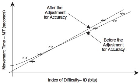
Figure 3 demonstrates the disparity between subjects' performance and the experimenter's intentions. Fitts' law models constructed without applying the adjustment for accuracy suffer from the problem that data points with very low ID values (i.e., close to the y-axis) tend to lie above the regression line. This is quite visible in Welford's plot of Fitts' original 1954 data. (Welford, 1960, Figure 6, on page 206) This upward curvature gives rise to a positive intercept value in regression models. This has caused some to suggest that Fitts' law does not apply in cases of low ID. (Gan & Hoffmann, 1988)²⁶ The solution to this problem is the adjustment for accuracy. Consider Figure 3a — instead of performing the easy task assigned, subjects are actually performing a significantly more difficult task — the effective target width is much smaller than the width of the target. The effective distance is also smaller than the prescribed distance, but the difference between We and W is much greater than the difference between De and D (i.e., We « W, while De < D). The net effect is to increase the effective index of difficulty (IDe > ID). Now consider what effect this has on a regression model. Without the adjustment for accuracy a regression model (using ID as the independent variable) must accommodate data points with positive MT values that are too close to the y-axis due to the underestimation of ID. This causes the low ID problem mentioned above — pushing the left extreme of the regression line (and hence the intercept) upwards. The adjustment for accuracy, on the other hand, places IDe values where they should be — in correspondence with the movement tasks that the subjects actually performed. See Figure 4.

Figure 4 - The effect of the adjustment for accuracy. This figure depicts the effect of the adjustment for accuracy on a regression model. Without the adjustment for accuracy, data points (marked with an '×') with low ID values are too near to the y-axis — and this artificially increases the y-intercept causing the data points to curve upwards from a straight line (we have bent the curve in this figure near the y-axis to illustrate this point). The arrows indicate the effect the adjustment for accuracy has on the data points. Low ID values are slightly increased while high ID values are slightly decreased, matching the subject's accuracy across all ID conditions. The net effect is to rotate the regression line counter-clockwise (reducing the intercept), and hence to correct the upward deviation of low ID data points above the regression line.

In the previous paragraph we noted that the discrepancy for low ID values was visible in a Figure in a paper by Welford. Later in the same paper Welford analyses the same data (from Fitts' 1954 paper) with the adjustment for accuracy and finds that the problem is corrected. (Welford, 1960, Figure 7, and see part "c)" on page 207; or see Welford, 1968, pages 146-148)²⁷ The beneficial effects of the adjustment for accuracy have been reported by others. For example, Card et al. after employing the adjustment for accuracy concluded that "all the points now lie on the line and the slight bowing has been corrected". (1983, pages 54-55) Fitts used the adjustment for accuracy in his later work (1964, page 110), concluding that "the corrected estimates of information rate... reveal a lower intercept but a higher slope constant". (1966, page 480) Elsewhere in the same paper Fitts' made the following complimentary comment about the adjustment for accuracy, "the authors feel that the data for the corrected estimates of task difficulty... provide a more precise estimate of information output, even though the range of values for [IDe] is thereby reduced and the correlations... are lower" (1966, page 479). MacKenzie has also found the adjustment for accuracy to be beneficial. (1989; 1991; 1992b)

In this section we provided arguments supporting recommendations III and IV — the need to measure the scatter of movement end-points (even if only in the form of error rates), and the necessity of applying the adjustment for accuracy. One may question the value of an experimental design where subjects are not able to conform to the task, and may be suspicious of data manipulations aimed at correcting this misbehaviour. But the adjustment for accuracy extends the range of ID values (particularly the low-ID range) over which Fitts' law may be applied. And of greater significance is that the adjustment for accuracy allows us to construct Fitts' law models that incorporate accuracy. Different subjects operate at different points in the speed-accuracy continuum, and consequently those who are more careful are more accurate but slower, and those who are more reckless are less accurate but faster. Without the adjustment for accuracy one does not have a complete picture of subjects' performance — the fast only appear faster, and the slow, slower. Small differences in accuracy are reconciled by the adjustment for accuracy. If the adjustment for accuracy introduces a very large difference between the ID and IDe, subject performance (both speed and accuracy) should be investigated and the reason for the large difference reported.

Next we have some brief comments concerning the formulation of the index of difficulty.

3.3 The Shannon Formulation of ID

The mathematical definition of index of difficulty has changed in the years since Fitts' 1954 paper. (1954) The preferred formulation, called the Shannon formulation (MacKenzie, 1989; MacKenzie, 1991; MacKenzie, 1992a), appears in Equation 1. The D and W terms measure distance, and commonly the units millimetres or pixels are used, while ID is measured in bits.²⁸

The superiority of the Shannon formulation over the two other popular formulations, those of Fitts (1954) and Welford (1960), is well documented. (MacKenzie, 1989; MacKenzie, 1991; MacKenzie, 1992a) The Shannon formulation is preferred because (i) it provides a better fit with observations (a higher correlation-coefficient is typically achieved), (ii) it exactly mimics the information theorem that Fitts' law is based on (Shannon & Weaver, 1949, theorem 17), and, (iii) with this formulation negative ID values are not possible.

Next, a few comments on linear regression are necessary.

3.4 Linear Regression and Fitts' law

Although linear regression is often used in conjunction with Fitts' law, linear regression is a mathematical procedure that is distinct from Fitts' law, with its own peculiarities and limitations. Given a set of n ordered pairs (x_i, y_i) one may find a straight line that describes the linear relationship between the independent (x_i) and dependent (y_i) data using the method of least squares. There are two properties of linear regression that are frequently overlooked in the context of Fitts' law: (i) it is not legitimate to make inferences outside the domain of the independent variable used to construct the regression model, and (ii) one may improve the correlation between observed data and a model by adding additional free variables (thus increasing the degrees of freedom of the model) but this comes with its own set of drawbacks.

Linear regression models are often used to interpolate y values for specific x values of interest; but this interpolation is limited to x values inside the domain of regression, in other words, inside the range [min(x_i) ... max(x_i)]. As an introductory text on statistics states...

"regression... is subject to misuses and misinterpretations... When making estimates from the regression equation, it's incorrect to make estimates beyond the range of the original observations. There's no way of knowing what the nature of the regression equation would be if we encountered values of the dependent variable larger or smaller than those we've observed". (Sanders, 1990, page 557)

This limitation of linear regression is particularly significant in the context of Fitts' law, as the literature shows that many researchers are interested in attaching a physical interpretation to the intercept. Note that the Shannon formulation for the index of difficulty cannot yield an ID value of zero bits or less, and will not produce ID values below 0.585 bits under the physical circumstances employed in most situations (i.e., so long as the starting position is outside of the target). This means that the y-intercept will always be outside of the domain of the independent data used in building the regression model. The reason given in the quotation above for limiting ourselves to the domain of regression is that the analysis has no information about what happens outside of the domain of regression. This argument hits right at the heart of the matter. What does it mean to make a rapid aimed movement where the distance of the movement is zero? Does Fitts' law even apply? The analogy of Fitts' law to Shannon's theorem 17 suggests that the intercept should be zero (the information capacity of a channel with no signal is zero).²⁹ The point made in the quotation is well-taken — it is not clear how Fitts' law should behave at the intercept, as there is no information regarding the low-ID region built into the regression model, because the intercept is outside of the domain of regression. So from the point of view of the regression model, it seems invalid to infer too much about the intercept. We will leave this point for the moment but will return to it again, in section 3.4.1.

The second property of linear regression mentioned above concerns the increased fit obtained using multiple regression by simply adding additional free variables (and thus increasing the degrees of freedom in the regression model). Regression models built from Fitts movement tasks typically produce coefficients of correlation (r) that are very high, usually greater than 0.900. (MacKenzie, 1992a, page 101) But this doesn't mean that higher correlations are not achievable; one merely has to introduce new free variables. For example, one common variant of Fitts' law that produces higher correlation values has three degrees of freedom, (MacKenzie, 1992a, page 105)

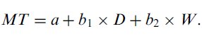
(14)

The hidden draw-back that occurs when we add free variables is that the meaning and influence of the parameters change, just as the meaning and values of the three parameters in Equation 14 do not align with the two parameters obtained from linear regression using Fitts' law. Consider the intercept of Equation 14 — it will take a different value than the Fitts' law regression intercept and does not have the same intuitive meaning (in fact its interpretation changes when D = 0 but W doesn't, when W = 0 but D doesn't, and when both W = 0 and D = 0). This is a compromise that researchers should be aware of; there are circumstances where very accurate models are warranted, but there are also situations where the effect the parameters have on one another is detrimental (two examples will be presented shortly).

The idea of the compromise between the fit of the model and its generality affects recommendations VI and VII. If Fitts' law is used to make movement time predictions, then researchers should take advantage of the better fit with observed data provided by linear regression (Equation 9). Conversely, if the purpose of the Fitts' law model is the comparison of conditions within an experiment, then the mean of means (Equation 10) should be used to calculate the dependent measure throughput. The reader may well question why linear regression (a two-degree of freedom model) should not be used to generate a dependent measure, why should the mean of means (a one-degree of freedom model) be used instead? After all, an alternate definition of throughput is possible; the reciprocal of the slope of the regression line, TP_Regression = 1/b, produces a measure that also has the units bits per second, and that at first glance appears quite similar to TP as defined in Equation 10 — but with a better fit to the data.

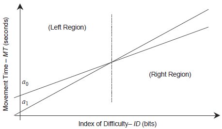
To address this question we refer the reader to Figure 5, a depiction of the comparison of two regression models. Two regression lines with differing slopes are presented. Because a₀ is less steep than a₁ the regression throughput for a₀, TP_Regression(a₀), defined as the reciprocal of the slope, is larger than that for a₁. To the casual observer this implies that a higher throughput was realised by subjects performing in the condition represented by line a₀. But this contradicts what is plainly apparent in Figure 5 — that the condition corresponding to a₀ was performed faster when the ID was high, but the a₁ condition was performed faster for low ID values. The reality is that these results are inconclusive. There is a contradiction here between what is plainly visible and the results according to TP_Regression. This contradiction is the result of the two-degree of freedom model used to calculate the slope — the slope coefficient of the regression model is unaffected by the high intercept of the a₀ condition (the whole point of using a two-degree of freedom model is to separate the effect of the intercept from the slope), and so it is not surprising that the regression throughput does not reflect the whole picture.

However, when throughput is defined so as to weigh the effect of all of the observations across all ID values equally, as Equation 10 does, we obtain a more accurate picture of performance. If Figure 5 depicted results of a real experiment, then the two lines would represent trends through two series of measured data points. And because the two lines (a₀ and a₁) cross at about their middles, we would expect the mean throughput of the data points corresponding to these lines to be approximately equal (both lines should have about the same spread of data points above and below the crossing point, otherwise the lines wouldn't cross at their middles). Thus the mean of the throughputs (Equation 10) would yield similar values for both conditions (a₀ and a₁), reflecting the fact that the average performance for both of these conditions was similar. This contrasts with the reciprocal of the regression slope (TP_Regression), which would suggest that there was a large difference between these two conditions (because the slopes of the lines are so different).

Figure 5 - Comparing two Fitts' law regression lines. This figure demonstrates the inconsistencies that arise when only the slope of linear regression values are used to compare performance. Note that the comparison of the two regression lines (a₀ and a₁) is inconclusive — for some ID values a₀ is better (produces a lower movement time), and for other ID values the converse is true. However, if the reciprocal of the regression slope was used to compare these conditions the experimenter would find that TP_Regression(a₀) > TP_Regression(a₁), falsely indicating that a₀ had a higher throughput. This contradiction arises precisely because a two-degree of freedom model is used — the intercept has no effect on the slope, and hence has no effect on the regression throughput statistic, TP_Regression.

This phenomenon is apparent when Fitts' (1954) 1-oz and 1-lb data are plotted together (not shown). Using Equation 10 (and the Shannon formulation, and the adjustment for accuracy), throughput values of 8.97 bps and 8.64 bps (respectively) result, suggesting that in Fitts' experiment the subjects performed the 1-oz condition 0.3 bps more efficiently (i.e., barely more efficiently) than the 1-lb condition. The reciprocal of the regression slope (TP_Regression), however, yields values of 8.20 bps and 7.20 bps respectively, exaggerating the difference between these two conditions.

One might wonder whether the reciprocal of the regression slope could be used in a study to test the hypothesis that a condition (A) is superior to another (B) for high ID values, but inferior for low ID values (as in Figure 5). TP_Regression cannot be used for this case either. The scientifically sound approach is to employ a two factor design, where condition (A or B) was one of the factors, and ID (high or low) was the other. Separate models would need to be constructed (four in total), using Equation 10 as the dependent measure, and a suitable ANOVA would have to be applied. In the absence of the application of proper scientific procedures, the results depicted in Figure 5 can do no more than merely suggest that such a relationship exists.

As another example consider Figure 6. Three regression models are depicted, all with identical slopes but different intercepts. If throughput is decoupled from the effect of the intercept (by using TP_Regression) then all three regression models depicted in Figure 6 appear equivalent, when clearly they are not.

Figure 6 - Regression models with identical slopes but different intercepts. Three regression models are depicted that demonstrate the need to incorporate the intercept into any dependent measure of performance. If these models were compared using only the reciprocal of the slope, they would all appear to be identical. Clearly, however, they are not. This is another example where throughput, as defined by Equation 10, performs properly, but the reciprocal of the regression line does not.

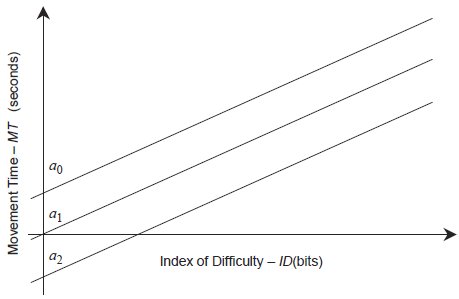
Again, throughput as defined by Equation 10 produces a result that is intuitive and correct. In Figure 6, the observed data points that gave rise to line a₀ would have a higher average movement time than data points on the next line down, a₁ (because a₀ is above a₁). Thus the throughput of the data points corresponding to a₀ will be lower (because the throughput of these data points is IDe_ij / MT_ij). And because throughput, as calculated via Equation 10, is the mean of the throughput of these data points, it too will be lower, reflecting the difference in performance between conditions a₀ and a₁, a difference that would be overlooked if the reciprocal of the regression slope (TP_Regression) was used instead.

Therefore we recommend the formulation in Equation 10 for the dependent measure throughput, to be used in the comparison of experimental conditions.

3.4.1 The physical interpretation of the intercept of the linear regression model

Much ado has been made of the intercept that occurs when applying linear regression to movement time data. Several interpretations have been offered, including:

i.		The time (possibly only theoretical) required to make a movement of zero distance (MacKenzie, 1992b, page 142), or the time for repetitive tapping "in-place" (Zhai, Sue, & Accot, 2002, page 22)
ii.		Unexplained secondary movement tasks, like the time for button presses (MacKenzie, 1992a, page 109), or dwell time (Fitts & Radford, 1966, page 476)
iii.		Unavoidable delay in the psychomotor system, extra feedback processing time (Fitts & Radford, 1966, page 476), uncontrollable muscle activity at the beginning or end of the movement task (MacKenzie, 1992a, page 109)
iv.		Reaction time (Fitts & Peterson, 1964, page 111)
v.		Modelling errors such as failing to use the Shannon formulation for ID, or failing to apply the adjustment for accuracy (MacKenzie, 1989; MacKenzie, 1991; MacKenzie, 1992a; Welford, 1960; Welford, 1968).

It has also been suggested that the intercept should be zero (or close to it) due to the intuitive reason that a movement rated at ID = 0 bits should not take any time to complete. (MacKenzie, 1992b, page 142) The opposite has also been suggested — Fitts noted the physical impossibility of a zero or less-than zero movement time, implying that the intercept should theoretically always be strictly positive. (1964, page 111; 1966, page 481)

Clearly, there is no consensus on the meaning of the intercept. Likely, the disagreement on the source of non-zero intercepts is the result of the fact that none of the explanations offered above are satisfactory. A particularly telling observation is that negative intercepts occur in the literature (for example, Fitts & Peterson, 1964, reports intercepts in the range -42 ms to -70 ms, page 107), and in some cases, quite large negative intercepts have been reported (for example, Epps, 1986, reported -587 ms; Kantowitz & Elvers, 1988, reported -880 ms). The existence of negative intercepts provides strong evidence that non-zero intercepts are not the result of secondary movements, delay in the psychomotor or biophysical systems of the body, or reaction time (explanations ii - iv above). When Fitts' original data were reanalysed by MacKenzie using the adjustment for accuracy and the Shannon formulation, -31.4 ms emerges as the intercept for the 1-oz stylus serial tapping task, and -69.8 ms for the 1-lb stylus task. (1992a, page 110) So explanations ii - v, above, are all unsatisfactory (and explanation i, above, does not apply in this case³⁰).

In our opinion, the most reasonable explanation for non-zero intercepts (barring a methodological problem, or lack of performing the proper analysis using the Shannon formulation including the adjustment for accuracy) is random variation in subject performance. Fortunately, this is easy to check for. We have performed a reanalysis of Fitts' data from his 1954 paper, and performed the statistical analysis described earlier in this paper to test whether the intercepts (for the 1-oz and 1-lb conditions) are significantly different from zero. For the 1-oz stylus task, the t-statistic is t = 2.353, and P(t ≥ T₁₄) = 0.0337. For the 1-lb stylus task, t = 4.209, and P(t ≥ T₁₄) < 0.01. Thus the evidence that Fitts' 1-oz task has a non-zero intercept is not strong (we can't say that the negative intercept is due to anything other than subject variation), but for the 1-lb task the intercept is significantly not zero. The negative intercept of the 1-lb task remains unexplained, but may be caused by subjects tiring from performing rapid movements with a stylus that weighs one pound, and thus taking a disproportionately long time, particularly on the more difficult tasks, thus tilting the regression line counter-clockwise, pushing the intercept negative. Nevertheless, the most likely cause of large non-zero intercepts are methodological problems,³¹ and the second most likely cause is subject variability.

3.4.2 The physical interpretation of the slope of the linear regression model

We have argued that the reciprocal of the slope of the regression model is not the same as the throughput, and has some disadvantages that make it unsuitable for use as a dependent measure. The slope is what it is — the component of the movement time that is explained by the change in ID, over the range of ID values used in building the model. The recommended dependent measure is throughput, calculated via the mean of means as per Equation 10.

3.5 The case for a low regression-intercept value

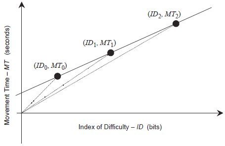
In a separate paper in this issue, Zhai (2004) argues that mean of means (Equation 10), and the direct division of mean scores³² produce measures of throughput that are not independent of the range of ID values employed by the experimenter. Figure 7 demonstrates this phenomenon. Three data points are displayed that fit a regression model with a substantial intercept, and between each of these and the origin we have drawn a dotted line. The steepness of the dotted lines is a function of how far to the right of the origin each data point is — the larger the ID, the lower the slope of the dotted line, and hence the higher the point-throughput³³ of that particular data point.

Figure 7 - The variation of throughput (TP) with ID. This figure illustrates the argument that non-zero intercepts introduce a systematic variance in the throughput values of each point, and that this variance depends upon ID. Observe that the throughput of each point (defined as ID_i / MT_i) amounts to the reciprocal of the slope of the dotted line that connects the point with the origin. The dotted lines each have different slopes, and hence each point has a different TP value that appears to increase for higher ID.

Zhai begins his analysis with a formulation for throughput that is similar to, but quite different from Equation 10, he writes,

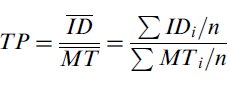
(15)

and then he substitutes MT_i = a + b × ID_i, yielding,

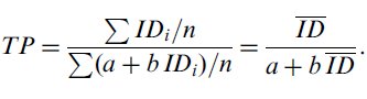
(16)

Zhai then argues that throughput is poorly defined because it depends upon a and b, and as such behaves poorly. One example provided of the poor behaviour of throughput is that it becomes undefined at the point ID = -a/b if the intercept is negative, due to division by zero. Zhai argues that the phenomenon depicted in Figure 7 makes throughput unsuitable for use as a dependent measure. This is an interesting point of view, but one that does not hold up under scrutiny. There are two reasons: (i) The mathematical substitution made by Zhai is not valid; it is the substitution that introduces the poor behaviour, not the definition of throughput. And, (ii) the alternative definition of throughput offered by Zhai, the reciprocal of the slope of the regression line, is no more independent of the range of ID values than throughput as defined by the division of means, nor the mean of means (Equation 10). These two points are elaborated next, followed by an analysis of Fitts' data demonstrating that the reciprocal of the slope (TP_Regression) varies with ID more than throughput as defined by Equation 10.

3.5.1 Invalid substitution

The claim that throughput (as defined by Equation 10) depends upon the coefficients of regression is false. Throughput depends upon only the effective index of difficulty, and the observed movement time — see Equation 10. The root of the problem in Zhai's analysis (Equations 15 and 16, above) lies in the invalid substitution of a + b × ID_i for MT_i in Equation 16. Just because one is willing to make this approximation does not mean that throughput actually does depend upon a and b. These coefficients (a and b) serve only as the parameters of the best fitting line through the data; a and b depend upon the observed data, the data do not depend upon a and b.

Consider this example. When regression is performed using Fitts' 1954 movement time data, using the Shannon formulation and the adjustment for accuracy, results consistent with MacKenzie's (1992a, page 110) reanalysis of Fitts' data are confirmed, yielding a coefficient of correlation of r = 0.9937. We performed linear regression of this same data against the second-order regression equation,

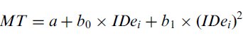
(17)

and achieved an even higher coefficient of correlation, r = 0.9947. Does this regression model, with its superior correlation, imply that throughput also depends on the term (IDe)²? No! To demonstrate a causal relationship between the regression coefficients and observed data requires an experiment where physical parameters equivalent to the coefficients (a and b) are treated as the independent variables, with observations that are statistically significant and, therefore, demonstrating that controlling those physical parameters (a and b) affects the data. The correlation between observed data and a linear regression model merely implies a linear relationship, no statement stronger this is possible without a controlled experiment.

The prediction of a regression model is not an acceptable substitute for real observed data. Real movement time data exhibit two properties that are absent in a regression model. (i) Observed data are variable. This allows the researcher to perform the adjustment for accuracy, and the adjustment for accuracy reduces the regression intercept — moving the y-intercept of the regression line close to the origin, thus minimising the disparity between the TP_Regression and TP as defined by Equation 10. (ii) Movement time observations in real data are always positive quantities — because time always moves forward. The aforementioned 'instability' where Zhai's formulae become ill-defined arises because Equation 16 suffers a division by zero (at ID = -a/b), which corresponds to a zero-second movement time). This behaviour does not occur when the correct mathematical formulation of throughput, Equation 10, is used. For Equation 10 to exhibit this same behaviour, a movement time of zero-seconds would have to be observed, and with real data this is impossible.

3.5.2 The reciprocal of the slope of the regression line is not independent of ID

Zhai's concern really reduces to the question of whether throughput depends upon the range of ID values used by the experimenter. It is apparent that Equation 10 contains the term IDe_ij, and hence throughput calculated via the mean of means depends upon ID. But the formulation for throughput preferred by Zhai also contains index of difficulty terms, and hence this formulation is not free of influence of ID either,³⁴

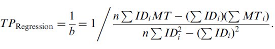
(18)

The real question is how these two formulations compare when real data are used, and it is this question that is addressed next.

3.5.3 A numerical example

Zhai presents an analysis using data from Card, English, and Burr (1978) wherein he pits the two formulations for throughput against one another and finds that the TP_Regression varies less with ID than throughput as defined here, by Equation 10. We feel this analysis is not very representative because the Card et al. data bears one of the largest regression intercept values (a = 1030 ms) in the published literature (this is apparent from Table 3, in section 4.1, upcoming in this paper). Consequently, this data exaggerates the difference between TP and TP_Regression. Frankly, this is not a reasonable intercept value — the implication is that when subjects performed a very easy movement task of little distance, they required more than one second to do so!

We replicated Zhai's analysis using data from Fitts' 1-oz task (from Fitts, 1954), and the results appear in Table 2.

Table 2
Comparison Of TP And TP_Regression Using Fitts' (1954) Data

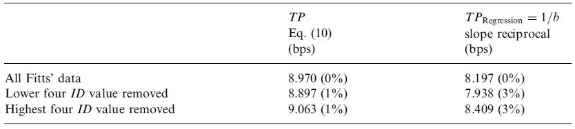
This table shows a reproduction of Zhai's analysis, but using the data from Fitts' (1954) paper, with the Shannon formulation for ID, and the adjustment for accuracy. The top line indicates the throughput values calculated using all of Fitts' data. The middle line shows the throughput values when the four lowest ID values have been omitted from the calculation (thus simulating the situation where the range of ID values used in the experiment was higher than it was). The bottom line shows the throughput values without the four highest ID values. The relative difference between the values is given in parentheses.

These results demonstrate that, so long as the data exhibit only a moderate regression intercept, the mean of means varies less with the index of difficulty than the reciprocal of the regression slope. And although the mean of means performs better, the variation due to ID is very small in both cases.

3.5.4 Further comments on TP versus TP_Regression

Regression models are useful tools given the right application, but we must avoid allowing regression to make us contemptuous of controlled observations. Consider Figure 7 again. If this figure depicted the results of a real experiment, then the experimenter would have a great deal of confidence in those three data points — after all, they would represent real observations made by a real witness. Somebody would have observed subjects performing at a throughput level of ID₀ / MT₀ during the first condition, ID₁ / MT₁ during the second, and ID₂ / MT₂ during the third. But since the results (Figure 7) have a positive intercept, the regression throughput (TP_Regression) yields a larger value than that observed during each of these three conditions. Regression cannot be allowed to annihilate observations.

Does the variation in TP apparent in Figure 7 imply that the range of ID values used in an experiment affects the final TP as defined by Equation 10? Possibly — but only if the intercept is very large. But even if the intercept is large the whole point of using TP as a dependent measure is that it encompasses the observations at all ID values. If a large positive intercept value is observed then (in the absence of a methodological problem) the experimenter observed that subjects performed with a higher point-TP value for higher ID movement tasks. But if the intercept is negative then the converse is true, subjects performed with a lower point-TP value for higher ID tasks. Regardless, these observations are accounted for in the preferred formulation for throughput (Equation 10) because it is an average of the observations. We must think about this the right way around — the effect of the intercept does not mean that we should throw-out throughput as a dependent measure, it means that we should exercise caution in choosing the range of ID values to present to subjects, and we should investigate thoroughly any large intercepts (whether positive or negative). In the end, we desire a statistic that is representative of the observed data, and the mean of means provides us with an average of the point-TP values over the conditions observed. Throughput is a well-defined and useful statistic (for further evidence to support this claim, see section 4.2, below). It is for these reasons that we make recommendations II, V, and VII, above. A wide range of ID values increases our confidence in the statistics and models constructed. A low intercept value decreases the variation of point-TP values, is theoretically desirable, and is achievable using the Shannon formulation for ID and the adjustment for accuracy.

3.6 Final comments on the justification of recommendations

The justification of the recommendations made earlier in this paper draws to a close. Arguments have been made supporting all seven recommendations. One feature of the published literature that was useful was the reanalysis of Fitts' original (1954) data, using the analysis techniques now available to us. This is only possible because Fitts included in his paper both movement time and error rate data. The utility of this aspect of Fitts' paper should not be overlooked — error rates are important and will be useful to future researchers who will, no doubt, have unimaginable new analysis techniques at their disposal. We wish to extend this reasoning to the distribution of movement end-point data as well. We recommend that movement times, error rates, average effective movement distances, and standard deviations of movement end-point locations, be included wherever possible in future papers reporting Fitts' law models, for each ID condition, for each subject.

4.0 The ISO standard versus Anarchy

In the introduction of this paper we claimed that HCI researchers would benefit from a standardized methodology with respect to Fitts' law. Here we present a very concise review of literature in the form of three tables and some brief comments. These tables demonstrate that the current state of the literature is inconsistent and contradictory, and hence not useful for researchers or practitioners that simply want to compare devices or use Fitts' law, without having to build their own models. The inconsistency and contradiction is a severe impediment to using Fitts' law in HCI. For example, in every new paper reporting experimental results, authors are obliged to write a line or two demonstrating that their results are consistent with the published body of work or explaining why their work is unique. But a look at the range of throughput values published over the years for the mouse assures us that no matter what throughput value one may measure in a study (no matter how flawed), one can still find a published paper that one's results can be said to be consistent with. The published literature exhibit too wide a variability in experimental methods and their results, and consequently the collected works are inconsistent with one another, contradictory, and not useful to the general practitioner.

The new ISO9241-9 standard, "Ergonomic requirements for office work with visual display terminals, Part 9: Requirements for non-keyboard input devices" officially became available in 2002, and nine studies have already been published using it (some no doubt using a draft of the standard). As we shall demonstrate, the contrast from the older studies is astonishing — consistency between studies (even studies performed by different research groups) is apparent. These mere nine studies are not enough to draw any strong conclusions from, but the results of these early adopters of the standard look promising. The review follows.

4.1 A review of 24 Fitts' law studies using the mouse

We have compiled a collection of 24 papers that present Fitts' law models for the mouse, and that do not use the ISO9241-9 standard. (Akamatsu, MacKenzie, & Hasbrouq, 1995; Boritz, Booth, & Cowan, 1991; Card et al., 1978; Douglas & Mithal, 1994; Epps, 1986; Gillan, Holden, Adam, Rudisill, & Magee, 1990; Gillan, Holden, Adam, Rudisill, & Magee, 1992; Guiard, Beaudouin-Lafon, & Mottet, 1999; Han, Jorna, Miller, & Tan, 1990; Hornof, 2001; Inkpen, 2001; Johnsgard, 1994; Jones, 1989; Jones, 1991; MacKenzie & Buxton, 1992; MacKenzie & Buxton, 1994; MacKenzie & Riddersma, 1994; MacKenzie, Sellen, & Buxton, 1991; MacKenzie & Ware, 1993; Miniotas, 2000; Mithal & Douglas, 1996; Po, Fisher, & Booth, 2004; Rutledge & Selker, 1990; Zhai, Conversy, Beaudouin-Lafon, & Guiard, 2003) The mouse is an ideal device to centre a survey like this around because it is the most common pointing device in use today and consequently is featured in more studies than any other pointing device. But there was also another motive in limiting ourselves to one device. Theoretically, the body of literature pertaining to a single device should present results that, while not identical, should be similar to one another. Although, as you will see, this is not the case.

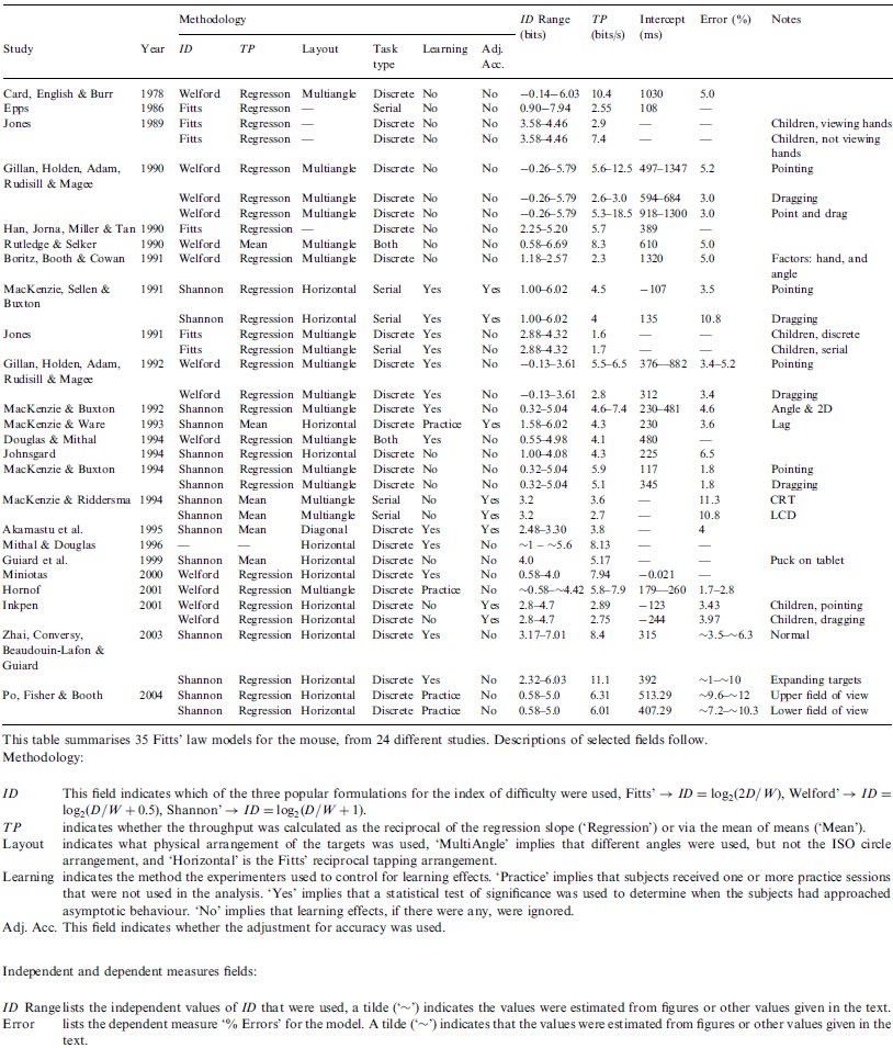
Our aim was to include all of the papers commonly available in the literature that present a Fitts' law model of the mouse. Many of these papers are investigations of devices other than the mouse and of conditions other than 'normal' mouse pointing — but they all build and publish a Fitts' law model for the mouse, even if just as a 'baseline' or control condition. Papers that use ID and measure movement times but that don't actually construct a Fitts' law model were not included (for example, Kabbash, MacKenzie, & Buxton, 1993). In cases where more than one Fitts' law model was included, the models occupy separate lines in the table (but in cases where the distinction between the models was slight and would have been uninteresting to the casual reader, we compressed them down to a single line). The papers appear in chronological order. See Table 3.

There are many models in this table that are supposed to represent 'normal' mouse pointing. One would think these models would demonstrate uniformity in their reported throughput values. However, if the reader scans down the 'Notes' column identifying models with either no notes, or where the notes read 'Pointing', and compares the throughput values reported for these models, a large range of TP values emerges for what should be similar tasks performed by similar devices. The lowest value for pointing with the mouse is 2.55 bits per second (bps) (Epps, 1986), and the highest value is 12.5 bps (Gillan et al., 1990). Although these two studies used similar ranges of ID, they used different formulations for ID, impeding our ability to compare them (yet another example of the need to use a consistent means to calculate and report Fitts' law models). But the disparity in TP values exists within groups with the same ID formulation as well; for the Fitts' formulation, 2.55 bps (Epps, 1986) and 5.7 bps (Han et al., 1990), for the Welford formulation, 2.3 bps (Boritz et al., 1991) versus 4.1 bps (Douglas & Mithal, 1994) versus 7.9 bps (Hornof, 2001) versus 10.4 bps (Card et al., 1978); and for the Shannon formulation, 4.5 bps (MacKenzie et al., 1991) compared with 8.4 bps (Zhai et al., 2003). These values contradict one other, and so are not useful to those who need a clear and accurate answer to the question, what is the throughput of the mouse?

The comparison of these studies is impeded by the multiplicity of conditions employed. Look at the 'Methodology ID' column — all three of the popular ID formulations are well represented. Note the inconsistency apparent in the ranges of ID values used in these studies.

One last observation we make of Table 3 concerns how few studies made use of the adjustment for accuracy, a technique that was first described by Crossman in 1957, and that Welford demonstrated as advantageous in 1960. Fitts himself even used the adjustment for accuracy, and wrote favourably about it, saying "the authors feel that the data for the corrected estimates of task difficulty... provide a more precise estimate of information output, even though the range of values for [IDe] is thereby reduced and the correlations... are lower" (1966, page 479)

The reader is encouraged to compare these results with the results in the next section of studies that used the ISO9241-9 standardised methodology.

Table 3
Survey Of Twenty-four Fitts' Law Studies Of The Mouse That Did Not Use The ISO 9241-9 Standard

4.2 A review of 9 Fitts' law studies conforming to ISO9241-9

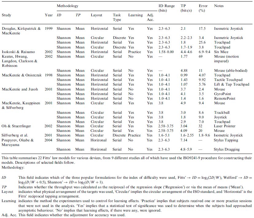
We have collected nine studies that used the procedure described in ISO9241-9 to build Fitts' law models. (Douglas et al., 1999; Isokoski & Raisamo, 2002; Keates et al., 2002; MacKenzie & Jusoh, 2001; MacKenzie et al., 2001; MacKenzie & Oniszczak, 1998; Oh & Stuerzlinger, 2002; Poupyrev et al., 2004; Silfverberg et al., 2001) Note that these nine studies are not all mice studies — a range of devices has been used. See Table 4.

From the first glance, the data in Table 4 appear much more uniform and consistent than Table 3. Not surprisingly, every study used the Shannon formulation, performed the adjustment for accuracy, and calculated throughput via the mean of means (as defined in Equation 10). An observation that is very promising is the narrowness of the ranges of throughput that appear in Table 4. In particular, consider the mouse throughput values. All of the throughputs fall in the range [3.7 - 4.9]. So, five different Fitts' law models (representing every publication with a mouse model available to us) from four separate research groups have published results that agree to within 1.2 bits per second (bps). Compare this to the almost 10 bps range of throughput values in Table 3.

Table 4
Survey Of Nine Studies That Used The ISO9241-9 Standard

The throughput range data from Table 4 is summarised in Table 5. As of yet there are too few ISO-conforming studies to conclude anything too strongly, but these studies support our contention that the advantage reaped, when researchers use consistent methods, is consistent results.

Table 5
Evidence Of Agreement In Throughput Values

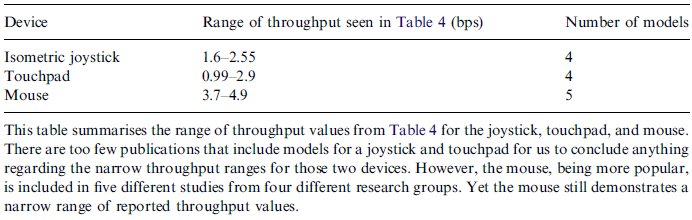
Note that the range of ID values that the mice studies in Table 4 used vary markedly. Isokoski & Raisamo (2002) used an ID range of 1.58 - 8.00 bits, MacKenzie & Jusoh (2001) used about half that range, 1.0 - 4.1 bits, Oh & Stuerzlinger (2002) used very narrow range of ID, 2.58 - 3.75 bits, and lastly, MacKenzie et al. (2001) used just one ID value, 3.8 bits. And yet the throughput values were surprisingly consistent across these ranges. If there is a systematic problem with throughput calculated via the mean of means (Equation 10) with regards to ID as discussed in section 3.5, it is not apparent here.

5.0 Conclusions

This paper is concerned with the theory and application of Fitts' law in HCI. Since its introduction in 1954, Fitts' relationship has been widely used in experimental psychology, human factors, and human-computer interaction. Attesting to its continued relevance are the many citations and adaptations of the model appearing each year in conference proceedings, journal articles, monographs, etc. In 1992, marking the centennial of the American Psychological Association, Fitts' original paper was reprinted in the Journal of Experimental Psychology. (Fitts, 1992) As Kelso noted in the preface to the reprint,

"There is little doubt that Fitts' (1954) work was a seminal article in the field: It was the first to apply Shannon and Weaver's (1949) theory of information to the motor system and to quantify task difficulty in terms of information units. In particular, the relation between amplitude, movement time, and precision (or tolerance) has come to be known as Fitts' law because of its wide applicability to different perceptual-motor tasks. Fitts was clearly committed to finding empirical relations that reflect limits of human capabilities, and the relation he identified has stood the test of time." (Kelso, 1992, page 260)

Fitts' law has only really "stood the test of time" if it continues to be useful and relevant. An inconsistently or incorrectly used model is hardly better than no model at all. We feel it is important to recognise that the HCI community has three choices with regards to Fitts' law. We can continue to allow the hodgepodge of variations of Fitts' law to be used for research and published in papers. We can embrace the ISO standard, update it, expand it, use it, and enforce it. Or we can come up with something new. But one way or another, meaningful progress in this field with regards to Fitts' law will be hampered until, one way or another, we all conform to a standard of some kind.

We have made seven recommendations to those who would use Fitts' law in HCI. They are:

I.		Use the Shannon formulation of ID (Equation 1) because it provides a better fit with observations, is truer to the information theorem that Fitts' law is based on, and because with this formulation a negative ID value is not possible.
II.		Use a wide range of ID values because it increases our confidence in the regression model produced, and increases the range of ID values that our regression model is valid over. The range 2 to 8 bits should apply to most situations.
III.		Measure the scatter of movement end-point positions as error rates or end-point position data (but preferably both). These data are necessary because they allow us to perform the adjustment for accuracy, and because in the absence of a measure of accuracy, speed measurements are meaningless.
IV.		Perform the adjustment for accuracy to transform the index of difficulty values into effective index of difficulty values. This ensures that the model reflects the performance that the subjects actually achieved. Any large discrepancy between the ID and IDe values should be investigated. Without the adjustment for accuracy researchers may experience problems modelling movement data with low ID values.
V.		Use linear regression of movement time and the effective index of difficulty to measure the goodness of fit (to decide whether Fitts' law indeed applies) and to verify that the intercept (a in Equation 5) is small. A small intercept is a useful check that one's experiment methodology is sound.
VI.		Limit predictions from the resulting Fitts' law model to the range of ID values that were used to construct the model. This is a limitation of linear regression, not of Fitts' law per se.
VII.		If devices or experiment conditions are to be compared, use throughput as a dependent measure and calculate it via the mean of means (Equation 10). Calculated this way, throughput is representative all of the observations, and not subject to the same limitations as the reciprocal of the intercept slope.

Further, we have presented detailed justifications for these seven recommendations. Lastly, we have argued for the adoption of a standard, to improve the quality and comparability of our models. The ISO9241-9 standard seems promising in this regard. A very condensed review of the literature was presented illustrating the chaos that exists when there is no standardisation, and suggesting that the ISO standard is already having a beneficial effect.

Acknowledgements

The authors would like to thank Shumin Zhai for participating in this discussion on the formulation of throughput. Academic debate is the life-blood of science; it is only by considering all points of view that progress can be made. We would also like to express our thanks to the reviewer and editors for their very helpful suggestions.

References

Akamatsu, M., MacKenzie, I. S., & Hasbrouq, T. 1995. A comparison of tactile, auditory, and visual feedback in a pointing task using a mouse-type device. Ergonomics, 38, 816-827.

Boritz, J., Booth, K. S., & Cowan, W. B. 1991. Fitts' law studies of directional mouse movement. Proceedings of Graphics Interface - GI '91, 216-223. Toronto: Canadian Information Processing Society.

Card, S. K., English, W. K., & Burr, B. J. 1978. Evaluation of mouse, rate-controlled isometric joystick, step keys, and text keys for text selection on a CRT. Ergonomics, 21, 601-613.

Card, S. K., Moran, T. P., & Newell, A. 1980. The keystroke-level model for user performance time with interactive systems. Communications of the ACM, 23(7), 396-410.

Card, S. K., Moran, T. P., & Newell, A. 1983. The psychology of human-computer interaction. Hillsdale, NJ: Hillsdale, NJ: Lawrence Erlbaum.

Crossman, E. R. F. W. 1957. The speed and accuracy of hand movements. In E. R. F. W. Crossman & W. D. Seymour (Eds.), The Nature and Acquisition of Industrial Skill.: Report to the MRC and DSIR Joint Committee on Individual Efficiency in Industry [unpublished].

Crossman, E. R. F. W. 1960. The information-capacity of the human motor-system in pursuit tracking. Quarterly Journal of Experimental Psychology, 12, 1-16.

Douglas, S. A., Kirkpatrick, A. E., & MacKenzie, I. S. 1999. Testing pointing device performance and user assessment with the ISO 9241, Part 9 standard. Proceedings of the ACM Conference on Human Factors in Computing Systems - CHI '99, 215-222. New York: ACM.

Douglas, S. A., & Mithal, A. K. 1994. The effect of reducing homing time on the speed of a finger-controlled isometric pointing device. Proceedings of the ACM Conference on Human Factors in Computing Systems - CHI '94, 411-416. New York: ACM.

Epps, B. W. 1986. Comparison of six cursor control devices based on Fitts' law models. Proceedings of the Human Factors Society 30th Annual Meeting - HFS '86, 327-331. Santa Monica, CA: Human Factors and Ergonomics Society.

Fano, R. M. 1961. Transmission of information: A statistical theory of communications: Cambridge, MA: MIT Press.

Fitts, P. M. 1953. The influence of response coding on performance in motor tasks. In B. McMillan (Ed.), Current trends in information theory (pp. 47-75). Pittsburgh, PA: University of Pittsburgh Press.

Fitts, P. M. 1954. The information capacity of the human motor system in controlling the amplitude of movement. Journal of Experimental Psychology, 47(6), 381-391.

Fitts, P. M. 1992. The information capacity of the human motor system in controlling the amplitude of movement. Journal of Experimental Psychology: General, 121(3), 262-269.

Fitts, P. M., & Peterson, J. R. 1964. Information capacity of discrete motor responses. Journal of Experimental Psychology, 67(2), 103-112.

Fitts, P. M., & Radford, B. K. 1966. Information capacity of discrete motor responses under different cognitive sets. Journal of Experimental Psychology, 71(4), 475-482.

Flowers, K. 1975. Handedness and controlled movement. British Journal of Psychology, 66, 39-52.

Gan, K.-C., & Hoffmann, E. R. 1988. Geometrical conditions for ballistic and visually controlled movements. Ergonomics, 31(5), 829-839.

Gillan, D. J., Holden, K., Adam, S., Rudisill, M., & Magee, L. 1990. How does Fitts' law fit pointing and dragging? Proceedings of the CHI '90 Conference on Human Factors in Computing Systems, 227-234. New York: ACM.

Gillan, D. J., Holden, K., Adam, S., Rudisill, M., & Magee, L. 1992. How should Fitts' law be applied to human-computer interaction? Interacting with Computers, 4(3), 291-313.

Glass, G. V., & Hopkins, K. D. 1996. Statistical Methods in Education and Psychology, Third Edition: Needham Heights, MA: Allyn & Bacon (Simon & Schuster Publishing).

Guiard, Y., Beaudouin-Lafon, M., & Mottet, D. 1999. Navigation as multiscale pointing: Extending Fitts' model to very high precision tasks. Proceedings of the ACM Conference on Human Factors in Computing Systems - CHI '99, 450-457. New York: ACM.

Han, S. H., Jorna, G. C., Miller, R. H., & Tan, K. C. 1990. A comparison of four input devices for the Macintosh interface. Proceedings of the Human Factors Society 34th Annual Meeting, 267-271. Human Factors Society.

Hornof, A. J. 2001. Visual search and mouse pointing in labeled versus unlabeled two-dimensional visual hierarchies. ACM Transactions on Computer-Human Interaction, 8(3), 171-197.

Inkpen, K. M. 2001. Drag-and-drop versus point-and-click mouse interaction styles for children. ACM Transactions on Computer-Human Interaction, 8(1), 1-33.

ISO. 2002. Reference Number: ISO 9241-9:2000(E):, Ergonomic requirements for office work with visual display terminals (VDTs) - Part 9 - Requirements for non-keyboard input devices (ISO 9241-9) (Vol. February 15, 2002): International Organisation for Standardisation.

Isokoski, P., & Raisamo, R. 2002. Speed-accuracy measures in a population of six mice. Proceedings of the Fifth Asia Pacific Conference on Human-Computer Interaction - APCHI 2002, 765-777. Bejing China: Science Press.

Johnsgard, T. 1994. Fitts' law with a virtual reality glove and a mouse: Effects of gain. Proceedings of Graphics Interface - GI '94, 8-15. Toronto: Canadian Information Processing Society.

Jones, T. 1989. Psychology of computer use: XVI. Effect of computer-pointing devices on children's processing rate. Perceptual and Motor Skills, 69, 1259-1263.

Jones, T. 1991. An empirical study of children's use of computer pointing devices. Journal of Educational Computing Research, 7(1), 61-76.

Kabbash, P., MacKenzie, I. S., & Buxton, W. 1993. Human performance using computer input devices in the preferred and non-preferred hands. Proceedings of the ACM Conference on Human Factors in Computing Systems - INTERCHI '93, 474-481. New York: ACM.

Kantowitz, B. H., & Elvers, G. C. 1988. Fitts' law with an isometric controller: Effects of order of control and control-display gain. Journal of Motor Behavior, 20, 53-66.

Keates, S., Hwang, F., Langdon, P., Clarkson, P. J., & Robinson, P. 2002. Cursor measures for motion-impaired computer users. Proceedings of the Fifth ACM Conference on Assistive Technology - ASSETS 2002, 135-142. New York: ACM.

Kelso, J. A. S. 1992. Theoretical concepts and strategies for understanding perceptual-motor skill: From information capacity in closed systems to self-organization in open, nonequilibrium systems. Journal of Experimental Psychology: General, 121(3), 260-261.

MacKenzie, I. S. 1989. A note on the information-theoretic basis for Fitts' law. Journal of Motor Behavior, 21, 323-330.

MacKenzie, I. S. 1991. Fitts' law as a performance model in human-computer interaction. Unpublished Doctoral Dissertation, University of Toronto (http://www.yorku.ca/mack/phd.html).

MacKenzie, I. S. 1992a. Fitts' law as a research and design tool in human-computer interaction. Human-Computer Interaction, 7, 91-139.

MacKenzie, I. S. 1992b. Movement time prediction in human-computer interfaces. Proceedings of Graphics Interface - GI '92, 140-150. Toronto: Canadian Information Processing Society.

MacKenzie, I. S., & Buxton, W. 1992. Extending Fitts' law to two-dimensional tasks. Proceedings of the ACM Conference on Human Factors in Computing Systems - CHI '92, 219-226. New York: ACM.

MacKenzie, I. S., & Buxton, W. 1994. Prediction of pointing and dragging times in graphical user interfaces. Interacting with Computers, 6(2), 213-227.

MacKenzie, I. S., & Jusoh, S. 2001. An evaluation of two input devices for remote pointing. Proceedings of the Eighth IFIP Working Conference on Engineering for Human-Computer Interaction - EHCI 2000, 235-249. Heidelberg, Germany: Springer-Verlag.

MacKenzie, I. S., Kauppinen, T., & Silfverberg, M. 2001. Accuracy measures for evaluating computer pointing devices. Proceedings of the ACM Conference on Human Factors in Computing Systems - CHI 2001, 9-16. New York: ACM.

MacKenzie, I. S., & Oniszczak, A. 1998. A comparison of three selection techniques for touchpads. Proceedings of the ACM Conference on Human Factors in Computing Systems - CHI '98, 336-343. New York: ACM.

MacKenzie, I. S., & Riddersma, S. 1994. Effects of output display and control-display gain on human performance in interactive systems. Behaviour & Information Technology, 13, 328-337.

MacKenzie, I. S., Sellen, A., & Buxton, W. 1991. A comparison of input devices in elemental pointing and dragging tasks. Proceedings of the ACM Conference on Human Factors in Computing Systems - CHI '91, 161-166. New York: ACM.

MacKenzie, I. S., & Ware, C. 1993. Lag as a determinant of human performance in interactive systems. Proceedings of the ACM Conference on Human Factors in Computing Systems - INTERCHI '93, 488-493. New York: ACM.

Miniotas, D. 2000. Application of Fitts' law to eye gaze interaction. Proceedings of the ACM Conference on Human Factors in Computing Systems - CHI 2000, 339-340. New York: ACM.

Mithal, A. K., & Douglas, S. A. 1996. Differences in movement microstructure of the mouse and the finger-controlled isometric joystick. Proceedings of the ACM Conference on Human Factors in Computing Systems - CHI 1996, 300-307. New York: ACM.

Newell, A., & Card, S. K. 1985. The prospects for psychological science in human-computer interaction. Human-Computer Interaction, 1, 209-242.

Oh, J.-Y., & Stuerzlinger, W. 2002. Laser pointers as collaborative pointing devices. Proceedings of Graphics Interface - GI 2002, 141-149. Toronto: Canadian Information Processing Society.

Plamondon, R., & Alimi, A. M. 1997. Speed/accuracy trade-offs in target-directed movements. Behavioural and Brain Sciences, 20, 279-349.

Po, B. A., Fisher, B., D., & Booth, K. S. 2004. Mouse and touchscreen selection in the upper and lower visual fields. Proceedings of the ACM Conference on Human Factors in Computing Systems - CHI 2004, 359-366. New York: ACM.

Poupyrev, I., Okabe, M., & Maruyama, S. 2004. Haptic feedback for pen computing: Directions and strategies. Extended Abstracts of the ACM Conference on Human Factors in Computing Systems - CHI 2004, 1309-1312. New York, NY: ACM.

Reza, F. M. 1961. An Introduction to Information Theory: New York, NY: McGraw-Hill.

Rutledge, J. D., & Selker, T. 1990. Force-to-motion functions for pointing. Proceedings of the Fourth IFIP Conference on Human-Computer Interaction - INTERACT '90, 701-706. Amsterdam: Elsevier Science.

Salmoni, A. W., & McIlwain, J. S. 1979. Fitts' reciprocal tapping task, a measure of motor capacity? Perceptual and Motor Skills, 49, 403-413. Sanders, D. H. 1990. Statistics: A Fresh Approach, Fourth Edition: McGraw-Hill: New York.

Schmidt, R. A., Zelaznik, H. N., & Frank, J. S. 1978. Sources of inaccuracy in rapid movement. In G. E. Stelmach (Ed.), Information processing in motor control and learning (pp. 183-203). New York: New York: Academic Press.

Sen, A., & Srivastava, M. 1990. Regression Analysis: Theory, Methods, and Applications: New York: Springer-Verlag.

Shannon, C. E., & Weaver, W. 1949. The mathematical theory of communication. Urbana, IL: University of Illinois Press.

Silfverberg, M., MacKenzie, I. S., & Kauppinen, T. 2001. An isometric joystick as a pointing device for handheld information terminals. Proceedings of Graphics Interface - GI 2001, 119-126. Toronto, Canada: Canadian Information Processing Society.

Soukoreff, R. W., & MacKenzie, I. S. 1995. Theoretical upper and lower bounds on typing speeds using a stylus and soft keyboard. Behaviour & Information Technology, 14(6), 370-379.

Soukoreff, W., & MacKenzie, S. 2002. Using Fitts' law to model key repeat time in text entry models. Poster Abstracts of Graphics Interface - GI 2002. (http://dynamicnetservices.com/~will/academic/).

Wade, M. G., Newell, K. M., & Wallace, S. A. 1978. Decision time and movement time as a function of response complexity in retarded persons. American Journal of Mental Deficiency, 83, 135-144.

Welford, A. T. 1960. The measurement of sensory-motor performance: Survey and reappraisal of twelve years' progress. Ergonomics, 3, 189-230.

Welford, A. T. 1968. Fundamentals of skill. London: London: Methuen.

Welford, A. T., Norris, A. H., & Shock, N. W. 1969. Speed and accuracy of movement and their changes with age. Attention and performance II [Acta Psychologica], 30, 3-15.

Woodworth, R. S. 1899. The accuracy of voluntary movement. Psychological Review (Series of Monograph Supplements), 3(No. 13), 1-114.

Zhai, S. 2004. Characterizing computer input with Fitts' law parameters - The information and non-information aspects of pointing. International Journal of Human-Computer Studies, In press.

Zhai, S., Conversy, S., Beaudouin-Lafon, M., & Guiard, Y. 2003. Human on-line response to target expansion. Proceedings of the ACM Conference on Human Factors in Computing Systems - CHI 2003, 177-184. New York: ACM.

Zhai, S., Sue, A., & Accot, J. 2002. Movement model, hits distribution and learning in virtual keyboarding. Proceedings of the ACM Conference on Human Factors in Computing Systems - CHI 2002, 17-24. New York: ACM.

---

Notes

^* Corresponding author. Email address: will@acm.org (R. W. Soukoreff).

¹ Note that Fitts' 1954 paper was reprinted in 1992 and this later version may be easier to obtain than the original. (Fitts, 1992)

² Plamondon and Alimi provide a brief review of the variety of circumstances where Fitts' law has been demonstrated to apply. These include different types of rapid aimed movement (i.e., serial tapping, dial rotation, object transferral), various parts of the body (fingers, hands, arms, feet, the head and the eyes), several physical circumstances (under a microscope, underwater), and a varied group of people (the young, aged, motor impaired, and drugged) (see Plamondon & Alimi, 1997, pages 281-282).

³ In the evaluation of a pointing device, many factors must be scrutinised including the ease and comfort with which the device may be used, the speed with which selections (or dragging tasks) can be performed, and the inherent accuracy of the device. But these features are not independent — ease and comfort can affect both the speed and the accuracy. And due to the speed-accuracy trade-off, speed and accuracy have opposing influences on each other. The practice in the literature is to measure and report several dependent measures, (subjective) ease and comfort, speed, accuracy, throughput, and any other pertinent measures. (For a description of other dependent measures relating to pointing device evaluation, see MacKenzie, Kauppinen, & Silfverberg, 2001.) Although this paper focuses on throughput as a dependent measure, speed and accuracy must both also be reported as separate dependent measures if one is to convey a complete picture of the performance of a device.

⁴ For the sake of being able to refer to these recommendations individually later in this paper, we have numbered each with a roman numeral.

⁵ In this section we have assumed the reader is familiar with the basic terms, formulae, and methodologies used with Fitts' law. These terms are explained in the justification section later in this paper.

⁶ Frequently in the literature the term A (amplitude) is used to represent the movement distance parameter in the formula for ID. We have used D instead, following the lead of the ISO standard.

⁷ Homing time refers to the time to move one's hand from the keyboard to the mouse and grasp it. Dwell time is used in some rehabilitation applications where, instead of clicking to indicate target selection, one must keep the pointing device within the bounds of one target (or icon) for a period of time to indicate selection. Neither homing time nor dwell time should be included in the movement time figures used to build a Fitts' law model. Reaction time only occurs with discrete tasks. It is the time from the onset of the stimulus to the beginning of movement.

⁸ Outliers often take the form of 'misfires' where the subject accidentally double-clicks on a target (registering an error for the following trial), or pauses mid-trial (violating the requirement that movements be rapid). As a guideline we recommend that any trials where the final movement distance or time is farther than 3 standard deviations away from the average should be investigated to determine whether they are outliers and removed if so.

⁹ This standard deviation should reflect the over-shoot or undershoot of the individual movements about the mean, in the direction of motion.

¹⁰ This calculation can be performed in Microsoft Excel with this formula: We = W * 2.066 / NORMSINV(1 − Err / 2), where W represents the width, and errors (Err) are stored as percentages (i.e., an error rate of 3.05% = 0.0305, not 3.05, and similarly, 0.0049% = 0.000049).

¹¹ Fitts' law only applies to rapid aimed movements — subjects that take their time compromise Fitts' law.

¹² This calculation should be performed combining all of the data (i.e., using all of the n pairs of movement time and index of difficulty data). This calculation can also be performed for each subject, if the experimenter is concerned about the quality of subjects' performance (i.e., to identify any subjects that violate Fitts' law by not making rapid aimed movements). Also, note that in this section we do not need to distinguish between the different subjects, and so we have simplified the subscripts of the IDe_ij and MT_ij terms to simply IDe_i and MT_i.

¹³ Unless the experimenter is investigating novice performance, subjects should be run through enough blocks of trials that they reach reasonably asymptotic (viz., expert) performance. Statistical tests (such as the Newman-Keuls, Scheffé or Tukey tests) exist to determine when this level of performance has been reached (see Glass & Hopkins, 1996, chapter 17).

¹⁴ This approach should be described in any statistics text with in-depth coverage of regression (for a detailed treatment see Sen & Srivastava, 1990, pages 14-18, and chapters 2 & 3, and in particular, section 3.5). Note also that the test for whether the intercept is statistically different from zero is called for often enough that many statistics packages provide this calculation automatically when performing linear regression calculations.

¹⁵ A two-tailed t-statistic should be used when calculating the p-value associated with the t-value, |a| / s.e.(a).

¹⁶ This is true because of the Shannon formulation of ID (Equation 1). The only way for ID to approach zero would be for either D to be zero, or W to become infinitely large. In both cases, Fitts' law does not apply.

¹⁷ This lack of a satisfactory psychomotor theory to explain Fitts' law is not due to a lack of trying. A recent paper by Plamondon and Alimi reviews eight such psychomotor models, and concludes that none of them adequately model or explain experimental observations. (1997, page 286). Plamondon and Alimi then propose their own kinematic model. Their paper includes an "Open Peer Commentary" section (Plamondon & Alimi, 1997, page 303-343) in which many other researchers observe deficiencies in the Plamondon and Alimi model. Thus, there is currently no satisfactory psychomotor model that explains Fitts' law. It is worth noting that Fitts concluded, since the results of his subjects using a 1-oz and 1-lb stylus were similar, that his relation was due to information processing instead of a physical mechanism. (1954, 390) Later comments suggested the he was content with the information theoretic interpretation of his law. (1964, page 110)

¹⁸ The variable W' appears in Shannon's work as W, we added the prime to Shannon's W to avoid confusing this parameter with the target width.

¹⁹ Any text on information theory will provide a detailed explanation. (For a rigorous treatment see: Fano, 1961, chapter 5; Reza, 1961, chapter 8; Shannon & Weaver, 1949, parts III and IV)

²⁰ We are being deliberately vague here — the signals can consist of any feature that can be measured such as, voltage, current, frequency, phase, or complicated combinations of any of the above. The physical manifestation of the signal and noise are irrelevant to our discussion here.

²¹ Two assumptions apply here, that the distribution of the signal is valid over the entire number line [−∞ ... ∞], and that the standard deviation of the distribution is specified.

²² Due to the speed-accuracy trade-off, people can affect their accuracy by manipulating their speed. (Salmoni & McIlwain, 1979, page 408; Schmidt, Zelaznik, & Frank, 1978, page 188; Woodworth, 1899, page 23-24) Further, several researchers have observed other factors that affect accuracy, including the distance moved, the accuracy required (viz., the target size), and the movement time allowed to subjects. (Fitts & Peterson, 1964; Kantowitz & Elvers, 1988; MacKenzie, 1992a; Salmoni & McIlwain, 1979; Schmidt et al., 1978; Wade, Newell, & Wallace, 1978; Welford, 1960; Welford, 1968; Woodworth, 1899)

²³ Crossman's 1957 paper is not widely available, but other authors have described the technique in detail, including Welford (Welford, 1960; Welford, 1968) and MacKenzie (MacKenzie, 1989; MacKenzie, 1991; MacKenzie, 1992a; MacKenzie, 1992b).

²⁴ Note that several researchers have observed that movement end-points conform to a Normal distribution. (Crossman, 1960; Fitts, 1954; Fitts & Radford, 1966; Flowers, 1975; Welford, Norris, & Shock, 1969)

²⁵ Note that Equation 3 treats the condition where the error rate is less than 0.0049% as a separate case. This is described by MacKenzie (1991, section 2.4; 1992a, page 108) as a "pragmatic" treatment for the condition where the error rate is zero. The term 0.5089 corresponds to z(p ≥ 98.060%) / z(p ≥ 1 - 0.0049% / 2).

²⁶ Note, however, that Gan and Hoffmann (1988) did not apply the adjustment for accuracy.

²⁷ Note that a second difference exists between Welford's two analyses — in the latter (adjusted for accuracy) analysis he employs a superior formulation for the index of difficulty. Welford notes that the new formulation of ID he uses does improve the discrepancy in the low ID range somewhat, but he still finds the adjustment for accuracy necessary. After applying the adjustment for accuracy, he in no uncertain terms, concludes that "the results lie close to a straight line which passes through the origin." (Welford, 1960, page 208; Welford, 1968, page 149)

²⁸ The units 'bits' arise because of the logarithm of base 2. The usual definition of a bit of information is the base 2 logarithm of the number of possible outcomes of an event. In Fitts' law we take a slight liberty with this definition — but one can imagine fracturing the movement space (D + W) into target-sized areas of uniform width (W), so the ratio ((D + W)/ W) represents the number of possible outcomes of the movement.

²⁹ Also, note that Shannon's theorem 17 has no intercept variable, see Equation 11.

³⁰ Additionally, note that the case of repetitive tapping in place is not well modelled by Fitts' law (see Soukoreff & MacKenzie, 2002).

³¹ We strongly recommend experimenters double-check the timing of their experiment software before running experiments. In most cases movement time should be measured from the time motion begins (thus excluding reaction time) until the moment that the subject begins to signal task completion (e.g., begins to push the mouse button). If task completion is achieved with a dwell time, the dwell time should not be counted as part of the movement time. Homing time (the time to move one's hand from the keyboard and grab the mouse) should similarly not be counted as part of movement time.

³² The direct division of mean scores corresponds to TP_{DirectDivision} = .

³³ Point-throughput is defined ID_i / MT_i, and for convenience is shortened to 'point-TP'.

³⁴ This formula is trivially derived from the formula for the slope coefficient in least-squares linear regression.