Topics

• "Investigation of a system by studying its analog has been fairly common in science; for example, in acoustics, the properties of various systems have been very successfully elucitated by setting up and studying the similar or analogous electrical system. Many students of physics will recall the most elementary explanation of electrical phenomena in terms of the more easily visualized but analogous hydraulic phenomena.
  It readily follows that an analog computer… operates by setting up an analogous system which is solved more easily but which is so similar to the real system that the solution is valid for both. An example of one of the oldest and most common of analog computers is the slide rule. Linear distance along each scale of the rule is proportional to the logarithm of the numbers engraved, and setting the slides for multiplication of two numbers is equivalent to summing the logarithms of the two numbers.
  Many analog computing elements are in everyday use, such as the watthour meter which continuously determines the product of electrical voltage and current to arrive at power in watts and then integrates this with respect top time to obtain the energy used in watt hours…
  The digital computer represents [ numbers ] as discrete digital numbers, whole numbers or decimal fractions. The analog computer represents mathematical quantities as an analogous continuous range of voltages…
  A second difference is in the method of solving a problem. Most digital computers perform only one arithmetic operation at a time, storing the result in memory and then proceeding to the next operation in the program. The analog computer performs all operations simultaneously. Thus it really operates as a simulator… The computer may frequently be operated on the same time scale as the real system being studied and the two may even be linked together… Since the operations are all performed simultaneously, the analog computer is faster than a digital computer of comparable cost. But tthis result is not obtained without some penalty…
  A digital computer is programmed by writing a set of instructions which will properly direct the computer at each step of the computation. The analog computer is programmed by interconnecting the various arithmetic units in such a way that the desired problem will be solved."
  [ from Lester S Skagg, Analog Computer Manual. U of Chicago, 1966, p. xii ]
• A K Dewdney has a very interesting article, "On the Spaghetti Computer and Other Analog Gadgets for Problem Solving" in Scientific American, 250(6):19-26, June 1984. Since this article is only available in the library, I will reprint here a few passages.
  "The essential delight of an analog computation lies in the notion that one is getting something for nothing. A problem that would require hours of computation by hand (or even by a digital computer) is solved by merely observing a physical system as it comes rapidly into equilibrium…"
  "Consider the DAG computer, or Spaghetti Analog Gadget. This device, in the configuration I have tested, is able to sort up to 700 numbers in order of decreasing magnitude. Sorting is a common task in digital computing, and algorithms for doing it have been highly refined, but the time needed to sort a list of numbers still grows somewhat faster than the size of the list. With SAG one must spend a little time setting up the machine for the particular list of numbers and a little more time reading out the results, but the actual sorting appears to take no time at all.
  Here is how SAG works. For each number in the sequence to be sorted, trim a piece of uncooked spaghetti to a length equal to the number. Naturally, appropriate units of measurement must be adopted. Now take all the pieces of trimmed spaghetti in one hand and, holding the bundle vertically and somewhat loosely, bring it down on a table rather sharply. The momentum of the individual rods ensures that all of them have one end resting on the table. In order to obtain the sorted sequence from the resting bundle, one has only to remove the tallest rod, then the tallest of the remaining rods and so on until the bundle is exhausted. As each rod is removed it is measured and the number is recorded…"
  "The next gadget in my collection computes the convex hull of n points in the plane. The convex hull is just the smallest convex region containing all the points. It is entirely defined by its boundary, a polygon that has one of the points at each vertex. The gadget that computes the boundary is made from a large board, some nails and a rubber band. I call it RAG, short for Rubber Band, Nails and Board Analog Gadget…
  To set up RAG simply drive n nails into the board at positions corresponding to the n points in the plane. Then pick up the rubber band, stretch it into a large circle surrounding all the nails and release it. The rubber band will snap into place, precisely defining the polygonal boundary of the convex hull."
  Another example is "the needle-sorter once widely used in libraries… In the needle-sorter a set of cards with notches and holes along one edge serves to show which books are due on a given day. The cards are stacked and a long needle is inserted into the hole corrsponding to that day. When the needle is lifted, only the cards with holes at that position come with it. The notched cards slip off the needle and remain in the stack."
  Dewdney's article includes several other examples, and it's well worth reading. An intriguing question is whether it is possible to implement the simplicity and speed of these analog solutions on digital machines.
• "There are two distinct families of computing device available to us today, the all pervasive digital computer and almost forgotten analog computer. These two types of computer operate on quite different principles.
  The digital computer is a sequential device, in general, operating on data one step at a time, in addition the digital computer represents data internally using a quite verbose but very robust form of representation called binary. Thus a single transistor in a digital computer can only store two states, on and off. Obviously to store a number to any sensible degree of precision, many transistors are required.
  An analog computer operates in a completely opposite way to the digital computer. For a start, all operations in an analog computer are performed in parallel, and secondly, data is represented in an analog computer as voltages, a very compact but not necessarily robust form of data. A single capacitor in an analog computer can represent one continuous variable."
  [ from Herbert M Sauro's Analog Computers ]
  "There is no restriction on the physical processes analog computers may utilize. Most common media are fluids and gases which can be made to vary in numerous dimensions." [ from Web Dictionary of Cybernetics and Systems ]
• "We found a small army of natural processes that were analogs of each other. The flow of electricity in a man-made circuit models the flow of heat. Waves in shallow water model shock waves in air. Soap bubbles model electric fields." This quote is from John H Lienhard's Old Analog Computer, a nice, short celebration of the Analog Facility, built by SwRI, Southwest Research Institute, in San Antonio, TX, in 1955.

   

  

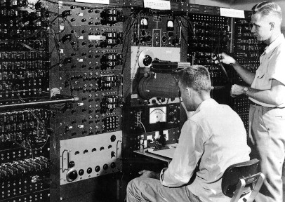
  SwRI Analog Design Facility for Pipeline Compressor Stations

   

• One of the essential components of electric and electronic analog computers is the operational amplifier, or op-amp. These devices, originally in the form of vacuum tubes and later as integrated circuits, date back from about 1947, and, as the term suggests, amplify or boost the amplitude of an input signal. They usually incorporate feedback, i.e. a fraction of the output is fed back to the input. See also Operational Amplifiers. where you can find "a K2-W tubes general purpose computing Op-Amp from George A. Philbrick Researches" (1952). They were developed to synthesize mathematical operations in analog computers. Here is an example from Doug Coward's Analog Computer Museum and History Center.

   

  

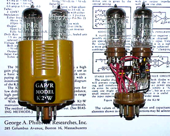
  K2-W General-Purpose Computing Op-Amp Tubes (1952)

   

• "A fully electronic general-purpose analog computer was designed by Helmut Hoelzer, a German electrical engineer and remote-controlled guidance specialist. He and an assistant built the device in 1941 in Peenemunde, Germany, where they were working as part of Wernher von Braun's long-range rocket development team. The computer was based on an electronic integrator and differentiator conceived by Hoelzer in 1935 and first applied to the guidance system of the A-4 rocket. This computer is significant in the history not only of analog computation but also of the formulation of simulation techniques. It contributed to a system for rocket development that resulted in vehicles capable of reaching the moon."
  [ from IEEE Annals of the History of Computing, July-September 1985 (Vol. 7, No. 3) ]
  Unlike digital computers (such as Zuse's Z machines), Nazi Germany seemd quite interested in analog computers.
• Of course analog computing devices have a very long history (see the exercise under 'Readings, Resources and Questions'). For example, in "1876-1878, Baron [ Lord ] Kelvin builds his harmonic analyzer and tide predictor machines. The harmonic analyzer broke down complex harmonic, or repeating, waves into the simpler waves that made them up. The tide predictor machine could calculate the time and height of the ebb and flood tides for any day of the year." [ from Kelvin's Tide Predictor ]

   

  

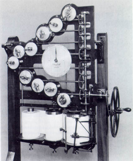
  Kelvin's Tide Predictor (1876-1878)

   

  A very interesting reference is The Tides, a lecture, delivered on Friday, August 25th, 1882 at the Southampton Meeting of the British Association, by William Thomson (Lord Kelvin) (1824 - 1907), in which he describes the reasons and the theory for building the tide predictor.
• As Williams notes [ op.cit., p. 201 ], "one of the problems that has vexed applied mathematicians over the years has been that of calculating the area under a given curve. This area, more formally known as the integral of the given function, or ∫ f(x)dx, is quite easy to calculate for elementary functions that can be integrated analytically, but can be almost impossible if the function, f(x), is either not known in analytic form or, if known, is not well behaved… It is quite easy to construct a mechanism such that, given a graph of y = f(x), you can have two pointers, one to run along the x axis of the graph and the other to follow the curve of y values." These devices were variously called integrators, planimeters, etc. See, for example, Computation without Electricity and Mechanical Integrator, part the Computer History Exhibits of Stanford's Computer Science Computer History Display.

   

  

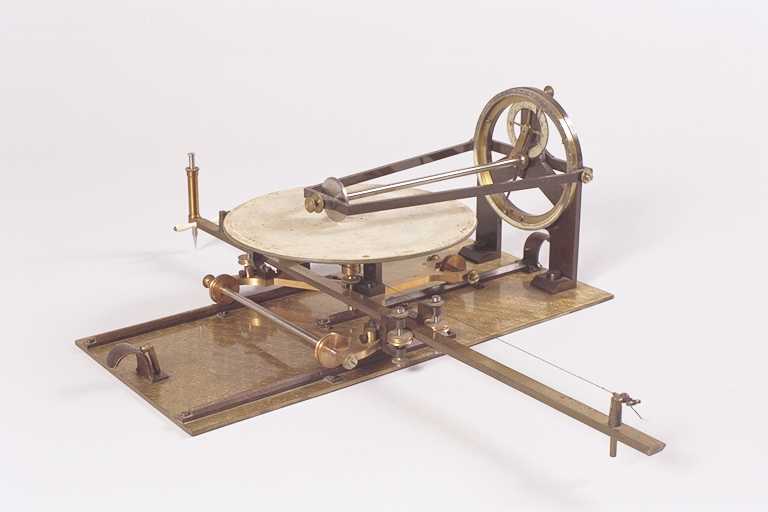
  G Starke's Planimeter (1849)

   

  "This instrument, invented by Jacob Amsler (1835-??) was used for computing the area enclosed by a closed curve. The arm OB ([ second ] figure below) has a pivot point in O which is fixed to the paper. In [ the ] Siemens planimeter, O is a sharp point pressed into the paper by a weight. Point B, which can describe a circle around O, rests in turn on a point of the arm AC. Point A is is moved by the user along the curve drawn on the paper. The other end of this arm rests on the paper with a steel wheel W, the axis of which is accurately parallel to AC. (In the Siemens planimeter, W is on the other side of A; also there is a supporting wheel perpendicular to W). The rotation of W can be measured accurately with the help of a division on its rim and a revolution counter. If AC is moved in its own direction, W slips over the paper without turning. However any movement component n normal to AC leads to a proportional rotation of W."

   

  

  Schematic Drawing of the Pole Planimeter

   

   

  

  The Basic Method for Computing Areas

   

  As Williams points out [ op. cit., p. 203 ], "the big drawback to incorporating this type of integrating device into any automatic calculating machinery was the fact that it relied simply on friction to drive the result wheel. If any tension was put on the result wheel, the contacts between the wheels and the rotating disks would slip., thus making the results invalid. The final solution to this problem was to devise some form of system to use the rotating result cylinder to control, but not actually drive, the gears and wheels used in the next stage of the process. The resulting system has been implemented in several different ways by different groups, but the first one to actually construct a working machine was Vannnevar Bush at MIT."
• One of the most important analog machines ever constructed was indeed Vannevar Bush's MIT Differential Analyzer, which he built in the early 1930s. "The machine was a completely mechanical assembly of gears and shafts driven by electric motors," and incorporated much refined planimeters.

   

  

  Vannevar Bush's Differential Analyzer

   

• Analog computers were used very soon to model, design and diagnose complex systems. See for example NASA's Flight and Analog Computer Study of Some Stabilization and Command Networks for an Automatically Controlled Interceptor During the Final Attack Phase, a report prepared in 1955.

   

  

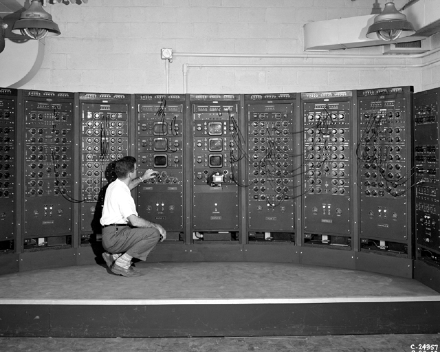
  Analog Computing Machine in Fuel Systems Building (NASA, 1949)

   

  Another, later example, is probably the largest analog computer ever built: The TRIDAC Analog Computer. TRIDAC stands for 'three-dimensional analogue computer,' as this machine (actually a building) was designed for solving problems of flight in three dimensions.

   

  

  The TRIDAC Analog Computer

   

  And here are a couple of examples of more recent machines. The first is in the the collection of the Computer Museum at the University of Amsterdam. The second at H Layer's Mind Machine Museum.

   

  

  Electronic Associates Inc. Model 680 Scientific Computing System (1968)

   

   

  

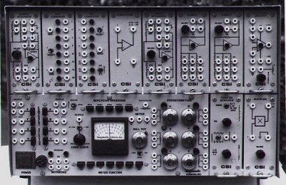
  Compumedic Analog Computer (1971)

   

• The University of Amsterdam's Computer Museum shows some actual examples of analog programming

   

  

  Representing the Dynamics of a Falling Body

   

  "The figure shows the set-up for the solution of a very simple second-order linear differential equation, representing the dynamics of a body moving (in one dimension) under the influence of gravity. Before the computation can be started, initial conditions (IC) must be specified. This is accomplished by charging the capacitors in both integrators to the voltages representing the zero-time velocity and position, respectively. On the patch panel a special IC input is provided for every integrator. By simply turning a console switch controlling the value of the integrating capacitors, the problem's time scale can be scaled up or down, making it suitable for plotting on a pen recorder, or for viewing on an oscilloscope. In the latter case the solution can be repeated quickly completely automatically."

 
Readings, Resources and Questions

• Browse all the previous lectures and identify the many examples of analog devices we have reviewed, even though we did not label them with the term 'analog.' Hint: the Antikythera Mechanism is a prime example.
• A very interesting and entertaining book is Analog Days: The Invention and Impact of the Moog Synthesizer, by Trevor Pinch and Frank Tocco (Harvard UP 2002). The authors promise (and deliver!) to "show that technology and cultural practices are deeply interwined."
• To get a sense of why analog computing is still very much of interest to scientists, look at Jonathan W Mill's 42 Questions about Analog Computing (don't worry about the technical details).
  Or read Analog Computer Trumps Turing Model, an article which briefly reviews Hava Siegelmann's work on analog computing at the Technion Institute of Technology, or the abstract of a paper, Computing Beyond Digital Computers by Neural Models, that Siegelman gave at the Hypercomputation Workshop at University College, London, in May 2000, where she and others go so far as claiming that "analog recurrent neural nets are, in general, more powerful than the universal Turing machine."